Plot the Survival Curve or CIF Dependent on a Continuous Variable as a 3D Surface

Using a previously fit time-to-event model, this function plots the survival curve as a function of a continuous variable using a 3D surface representation. This function can produce interactive plots using the plotly package, or a static image using the persp function of the graphics package.

Usage

plot_surv_3Dsurface(time, status, variable, data, model,
                    cif=FALSE, na.action=options()$na.action,
                    horizon=NULL, fixed_t=NULL, max_t=Inf,
                    interactive=FALSE,
                    xlab="Time", ylab="Survival Probability",
                    zlab=variable, ticktype="detailed",
                    theta=120, phi=20, col="green", shade=0.5,
                    ...)

Arguments

time: A single character string specifying the time-to-event variable. Needs to be a valid column name of a numeric variable in data.
status: A single character string specifying the status variable, indicating if a person has experienced an event or not. Needs to be a valid column name of a numeric or logical variable in data.
variable: A single character string specifying the continuous variable of interest, for which the survival curves should be estimated. This variable has to be contained in the data.frame that is supplied to the data argument.
data: A data.frame containing all required variables.
model: A model describing the time-to-event process (such as an coxph model). Needs to include variable as an independent variable. It also has to have an associated predictRisk method. See ?predictRisk for more details.
cif: Whether to plot the cumulative incidence (CIF) instead of the survival probability. If multiple failure types are present, the survival probability cannot be estimated in an unbiased way. This function will always return CIF estimates in that case.
na.action: How missing values should be handled. Can be one of: na.fail, na.omit, na.pass, na.exclude or a user-defined custom function. Also accepts strings of the function names. See ?na.action for more details. By default it uses the na.action which is set in the global options by the respective user.
horizon: A numeric vector containing a range of values of variable for which the survival curves should be calculated or NULL (default). If NULL, the horizon is constructed as a sequence from the lowest to the highest value observed in variable with 40 equally spaced steps.
fixed_t: A numeric vector containing points in time at which the survival probabilities should be calculated or NULL (default). If NULL, the survival probability is estimated at every point in time at which an event occurred.
max_t: A number indicating the latest survival time which is to be plotted.
interactive: Whether to draw the 3D surface as a static plot (interactive=FALSE, the default) or as an interactive plot. When interactive=TRUE is used, this function relies on the plotly package. In this case, the only aesthetic arguments that still work are the xlab, ylab and zlab arguments. Everything else has to be set manually using the functionality of the plotly package directly.
xlab: A character string used as the x-axis label of the plot, representing the survival time.
ylab: A character string used as the y-axis label of the plot, representing the survival probability or CIF.
zlab: A character string used as the z-axis of the plot, representing the continuous covariate of interest.
ticktype: A single character: "simple" draws just an arrow parallel to the axis to indicate direction of increase; "detailed" draws normal ticks as per 2D plots. Passed to the ticktype argument in the persp function. Ignored if interactive=TRUE.
theta: Angles defining the viewing direction. theta gives the azimuthal direction and phi the colatitude. Passed to the theta argument in the persp function. Ignored if interactive=TRUE.
phi: See argument theta. Passed to the phi argument in the persp function. Ignored if interactive=TRUE.
col: The color(s) of the surface facets. Transparent colours are ignored. This is recycled to the (nx-1)(ny-1) facets. Passed to the col argument in the persp function. Ignored if interactive=TRUE.
shade: The shade at a surface facet is computed as ((1+d)/2)^shade, where d is the dot product of a unit vector normal to the facet and a unit vector in the direction of a light source. Values of shade close to one yield shading similar to a point light source model and values close to zero produce no shading. Values in the range 0.5 to 0.75 provide an approximation to daylight illumination. Passed to the shade argument in the persp function. Ignored if interactive=TRUE.
...: Further arguments passed to curve_cont.

Details

The survival curve or CIF dependent on a continuous variable can be viewed as a 3D surface. All other plots in this package try to visualize this surface by reducing it to two dimensions using color scales or summary statistics. This function on the other hand directly plots the 3D surface as such.

Although 3D plots are frowned upon by many scientists, it might be a good visualisation choice from time to time. Using the interactive=TRUE option makes the plot interactive, which lessens some of the valid criticism of 3D graphics. Similar looking plots for the same purpose but using a likelihood-ratio approach have been proposed in Smith et al. (2019).

Value

Returns a plotly object if interactive=TRUE is used and a matrix when interactive=FALSE is used (still drawing the plot).

Author

Robin Denz

References

Smith, A. M.; Christodouleas, J. P. & Hwang, W.-T. Understanding the Predictive Value of Continuous Markers for Censored Survival Data Using a Likelihood Ratio Approach BMC Medical Research Methodology, 2019, 19

Examples

library(contsurvplot)
library(riskRegression)
library(survival)
library(splines)
library(ggplot2)
library(plotly)
#> 
#> Attaching package: ‘plotly’
#> The following object is masked from ‘package:ggplot2’:
#> 
#>     last_plot
#> The following object is masked from ‘package:stats’:
#> 
#>     filter
#> The following object is masked from ‘package:graphics’:
#> 
#>     layout

# using data from the survival package
data(nafld, package="survival")

# take a random sample to keep example fast
set.seed(41)
nafld1 <- nafld1[sample(nrow(nafld1), 150), ]

# fit cox-model with age
model <- coxph(Surv(futime, status) ~ age, data=nafld1, x=TRUE)

# plot effect of age on survival for ages 50 to 80
plot_surv_3Dsurface(time="futime",
                    status="status",
                    variable="age",
                    data=nafld1,
                    model=model,
                    horizon=seq(50, 80, 0.5),
                    interactive=FALSE)


# plot effect of age on survival using an interactive plot for ages 50 to 80
plot_surv_3Dsurface(time="futime",
                    status="status",
                    variable="age",
                    data=nafld1,
                    model=model,
                    horizon=seq(50, 80, 0.5),
                    interactive=TRUE)


## showing non-linear effects

# fit cox-model with bmi modeled using B-Splines,
# adjusting for age
model2 <- coxph(Surv(futime, status) ~ age + bs(bmi, df=3),
                data=nafld1, x=TRUE)

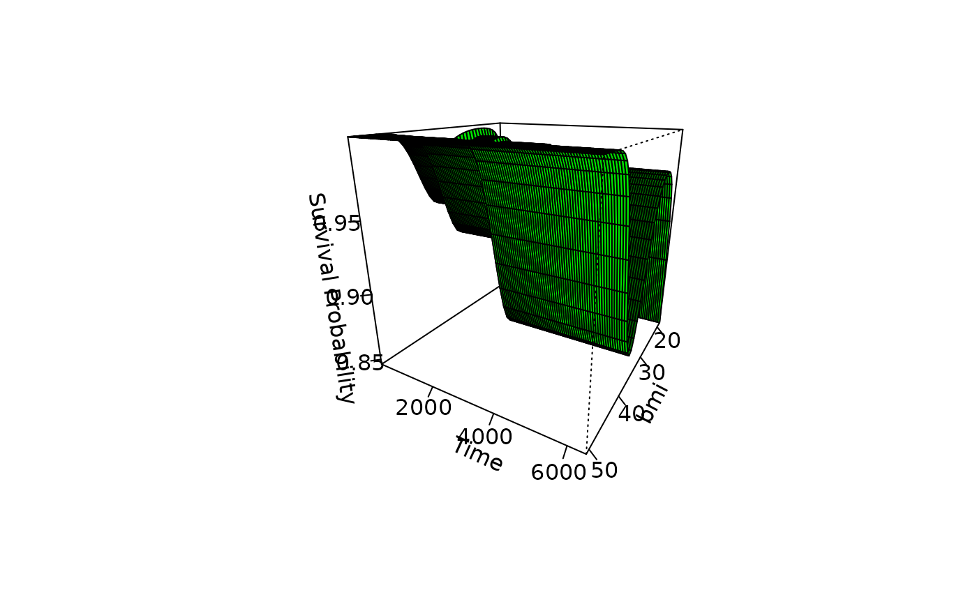
# plot effect of bmi on survival using normal plot
plot_surv_3Dsurface(time="futime",
                    status="status",
                    variable="bmi",
                    data=nafld1,
                    model=model2,
                    interactive=FALSE)


# plot effect of bmi on survival using interactive plot
plot_surv_3Dsurface(time="futime",
                    status="status",
                    variable="bmi",
                    data=nafld1,
                    model=model2,
                    interactive=TRUE)