Plot the time under observation for ids in a match_time object

Given a match_time object created using the match_time function, this plot_timeline function displays the time under observation of ids in relation to an event added using the add_outcome function. This function may be used to visually explain the matching process or the used censoring method.

Usage

plot_timeline(x, include, id_type=x$id, time_name,
              status_name, treat_point=TRUE,
              outcome_point=TRUE, next_treat_point=TRUE,
              linetype="solid", linewidth=1,
              size=3, shape_treat=18, shape_outcome=16,
              shape_next_treat=8, xlab="Time",
              ylab=".id_new", legend.position="right",
              gg_theme=ggplot2::theme_bw(), warn=TRUE)

Arguments

x: A match_time object created using the match_time function.
include: An optional numeric vector of ids that should be displayed in the plot. If this argument is not specified, the timelines for all .id_new in the matched data will be displayed. Even for small sample sizes this might not be the best option, which is why a warning message is returned by default if warn=TRUE. Which of the three possible ids in x$data should be used should be specified using the id_type argument.
id_type: There are three id variables in x$data: x$id (the original person identifier), .id_new (an id identifying separate rows in the final matched data) and .id_pair (an id identifying the matched pairs). By specifying this argument, users can choose which ids the include argument refers to. The y-axis will always display the .id_new id, but the plot will only include the ids mentioned in include of type id_type.
time_name: A single character string, specifying the name of a time-to-event variable added to x using the add_outcome function. This event time will be used as the end of the id specific timeline.
status_name: A single character string, specifying the name of the status of a time-to-event variable added to x using the add_outcome function.
treat_point: Either TRUE or FALSE, specifying whether a point should be added whenever a person received the treatment at inclusion time (essentially marking all cases).
outcome_point: Either TRUE or FALSE, specifying whether a point should be added whenever a person experiences an event.
next_treat_point: Either TRUE or FALSE, specifying whether a point should be added whenever a person receives the treatment after being included during the matching process.
linetype: A single character string specifying the linetype of the displayed lines.
linewidth: A single number specifying the width of the displayed lines.
size: A single number specifying the size of the drawn points (if any).
shape_treat: The shape of the point drawn if treat_point=TRUE.
shape_outcome: The shape of the point drawn if outcome_point=TRUE.
shape_next_treat: The shape of the point drawn if next_treat_point=TRUE.
xlab: A single character string specifying the label of the x-axis.
ylab: A single character string specifying the label of the y-axis.
legend.position: A single character string specifying the position of the label.
gg_theme: A ggplot2 theme to be added to the plot.
warn: Either TRUE or FALSE, specifying whether a warning should be printed if include is not specified.

Author

Robin Denz

Details

The displayed timelines always start at the "time-zero" defined by the matching process (.treat_time in x$data). How far the lines extend depends on the argument used when calling the add_outcome function.

Value

Returns a ggplot2 object.

Examples

library(data.table)
library(MatchTime)

# only execute if packages are available
if (requireNamespace("survival") & requireNamespace("ggplot2") &
    requireNamespace("MatchIt")) {

library(survival)
library(ggplot2)
library(MatchIt)

# set random seed to make the output replicably
set.seed(1234)

# load "heart" data from survival package
data("heart")

# perform nearest neighbor time-dependent matching on "age" and "surgery"
# (plus exact matching on time)
out <- match_time(transplant ~ age + surgery, data=heart, id="id",
                  match_method="nearest", replace_over_t=TRUE)

# suppose we had an extra dataset with events that looks like this
# NOTE: these are not all events in the real "heart" data and is merely used
#       for showcasing the functionality of add_outcome()
d_events <- data.table(id=c(1, 2, 3, 4, 5, 6, 7, 8, 9, 10),
                       time=c(50, 6, 16, 39, 18, 3, 675, 40, 85, 58))

# add the outcome to the match_time object
out <- add_outcome(out, data=d_events, time="time", censor_at_treat=TRUE)

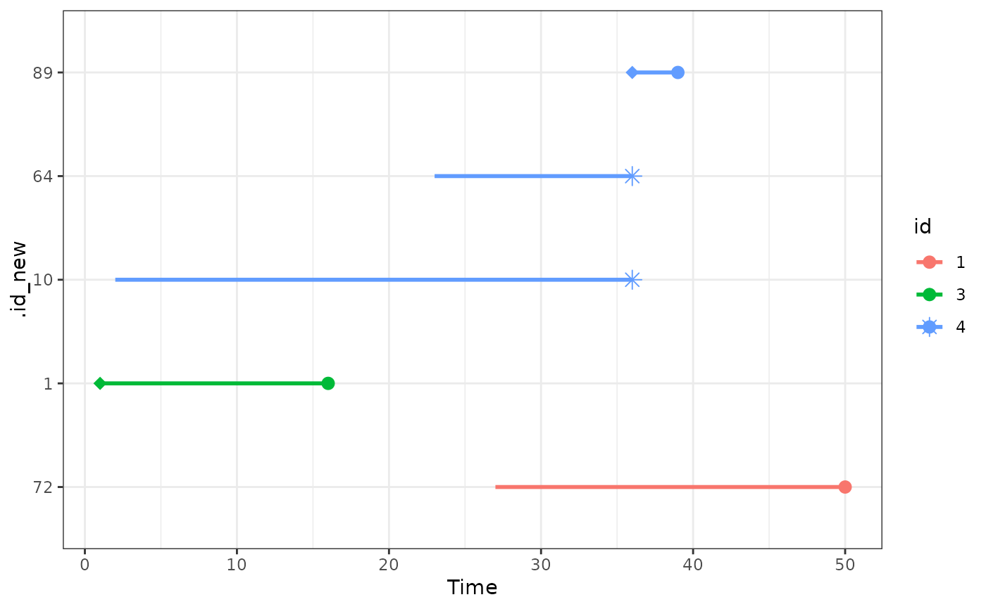
# plot the timeline for the original ids
# NOTE: here we see that id = 4 occurs 3 times in the matched dataset
#       1.) as a case, starting from ~ t = 36 (.id_new = 89)
#       2.) as a control, starting from ~ t = 23 (.id_new = 63)
#       3.) as a control, starting from ~ t = 2 (.id_new = 5)
#       This is possible because replace_over_t=TRUE was used
plot_timeline(out, include=c(1, 2, 3, 4, 5),
              time_name=".event_time", status_name=".status")
}
#> Warning: glm.fit: algorithm did not converge
#> Warning: glm.fit: fitted probabilities numerically 0 or 1 occurred
#> Warning: glm.fit: fitted probabilities numerically 0 or 1 occurred
#> Warning: glm.fit: algorithm did not converge
#> Warning: glm.fit: fitted probabilities numerically 0 or 1 occurred
#> Warning: glm.fit: algorithm did not converge
#> Warning: glm.fit: fitted probabilities numerically 0 or 1 occurred
#> Warning: glm.fit: algorithm did not converge
#> Warning: glm.fit: fitted probabilities numerically 0 or 1 occurred
#> Warning: glm.fit: algorithm did not converge
#> Warning: glm.fit: fitted probabilities numerically 0 or 1 occurred
#> Warning: glm.fit: algorithm did not converge
#> Warning: glm.fit: fitted probabilities numerically 0 or 1 occurred

Plot the time under observation for ids in a `match_time` object