An Introduction to Time-Dependent Matching with MatchTime

Introduction

Time-dependent matching is a very versatile method to perform causal inference based analysis with longitudinal data. In this type of matching, individuals who switch from “control” to the “treatment” at some point in time $t$ are matched to one or more (usually similar) individuals who are still under “control” conditions at $t$ . This point in time is then used as the “baseline” or “time-zero” for all individuals included in this way. The time from this artificial inclusion time until the occurrence of some time-dependent event is then usually used as an outcome, mimicking a prospective randomized controlled trial with staggered entry of participants (Thomas et al. 2020). There are multiple different versions of time-dependent matching that follow these general principles, such as balanced risk set matching (Li et al. 2001), time-dependent propensity score matching (Lu 2005), time-dependent prognostic score matching (Hansen 2008; He et al. 2020), time-dependent double-score matching (He et al. 2020) and time-dependent greedy matching (Gran et al. 2010). More information about the methods themselves is given in the documentation pages and the cited literature. To get a general overview, we also highly recommend the excellent review article by Thomas et al. (2020).

The MatchTime package aims to implement all forms of time-dependent matching for binary treatment variables in a consistent fashion. The package is designed to be as similar as possible to the MatchIt package (Ho et al. 2011), which is probably the most widely used piece of software to conduct regular matching (without time-dependent treatments). In fact, since most time-dependent matching methods require regular matching at each considered point in time, the MatchTime package has built-in support for MatchIt (Ho et al. 2011) and all of its’ functionality. This vignette gives a first small introduction to the general workflow when using MatchTime.

library(MatchTime)
library(data.table)
library(survival)
library(MatchIt)
library(cobalt)

An Example: The Stanford Heart Transplant Program

To better illustrate the features of this package, we will re-analyze real data that is publicly available. In particular, we will use the heart dataset from the famous survival R package here. Contrary to other packages implementing forms of time-dependent matching, the MatchTime package requires the input data to be in the start-stop format. This means that for each individual, all information should be encoded in form of time intervals in which the value of the included covariates does not change. This allows users to perform the matching in discrete and continuous time, without any need for equally spaced times of measurement. A more detailed explanation is given in the documentation pages and the associated vignette (see vignette("creating_start_stop_data", package="MatchTime")).

The heart dataset can be accessed using:

data("heart", package="survival")

This dataset has been pre-processed to be in the start-stop format and contains information of 103 patients on the waiting list for the Stanford heart transplant program (Crowley and Hu 1977). The first few rows of the data look like this:

head(heart)

##   start stop event        age      year surgery transplant id
## 1     0   50     1 -17.155373 0.1232033       0          0  1
## 2     0    6     1   3.835729 0.2546201       0          0  2
## 3     0    1     0   6.297057 0.2655715       0          0  3
## 4     1   16     1   6.297057 0.2655715       0          1  3
## 5     0   36     0  -7.737166 0.4900753       0          0  4
## 6    36   39     1  -7.737166 0.4900753       0          1  4

In this dataset, the columns called start and stop are used to define the right-open time-intervals, while the id column is used to identify which rows belong to which individual. The event column contains the binary event indicator that is 0 if no event occurred and 1 if an event occurred exactly at the stop value. Additionally, the dataset contains four covariates, age (the age of the individual in years - 48 years), the year of acceptance (in years after the first November 1967), surgery (whether the person had a prior bypass surgery) and whether the person received a transplant or not.

Here, individual with id = 1 has never received a transplant and experienced an event after 50 time units. Since no covariate values change for this person, he or she only has one row in the dataset. The individual with id = 4 on the other hand received a transplant at $t = 36$ and experienced an event three time units later at $t = 39$ with no other covariate changes inbetween. He or she therefore occupies two rows in this dataset.

For exemplary purposes, we will use the transplant variable as the treatment we are interested in and will consider the three other covariates (age, years and surgery) as confounders. We will pretend that the goal is to estimate the causal effect of the transplant on the event. Since transplant is a binary time-varying variable and the dataset is already in the required format, this is a neat example to introduce the capabilities of MatchTime. The results should, however, not be taken too seriously as the analysis is only performed for pedagogical purposes.

Performing the Matching

We can perform balanced risk set matching using nearest neighbor matching at each point in time using the following match_time() call:

set.seed(12345)

m_out <- match_time(transplant ~ age + surgery,
                    id="id",
                    outcomes="event",
                    data=heart,
                    method="brsm",
                    match_method="nearest",
                    replace_over_t=TRUE)
m_out

## A match_time object
##  - method: balanced risk set matching
##  - match-method: 1:1 nearest neighbor matching (using matchit())
##  - controls: Replacing controls only over time
##  - cases: Using all cases
##  - number of obs.: 103 (original), 138 (matched)
##  - target estimand: ATT
##  - covariates: age, surgery

Here, we first set a seed for the pseudo-random number generator to make the results replicable. This is required, because the selection of controls is based on randomness. Afterwards we can directly call the main function of this package to do the matching for us. The formula argument is used to define what parts of data should be matched. We define the treatment variable by putting it on the LHS of the formula and the confounders to be matched on by putting them on the RHS. Since there are multiple rows per person, we also have to tell the function how to identify these persons using the id argument. Additionally, we use the outcomes argument to specify which variables should be coded as time-to-event outcomes to allow an easier analysis later.

Next, the method argument controls the time-dependent matching method, which is set to balanced risk set matching (Li et al. 2001) here, while the match_method argument specifies the actual matching algorithm used when matching controls to the cases at each point in time. Here we set match_method="nearest", which means that nearest neighbor matching, as implemented in MatchIt::matchit() will be used. Finally, we set replace_over_t=TRUE to allow controls to be re-used over multiple points in time. Note that, similar to matchit(), each method may have additional arguments or caveats that are documented in their own documentation page.

Inspecting and Visualizing the Matching Process

Because the match_time() function basically does everything automatically, it might be difficult to understand what exactly actually happened at first. Luckily, the MatchTime package includes multiple functions to visualize the matching process and the results.

First, it always makes sense to take a look at the number of matches and controls throughout the matching process. This can be done easily using the plot.match_time() function:

plot(m_out)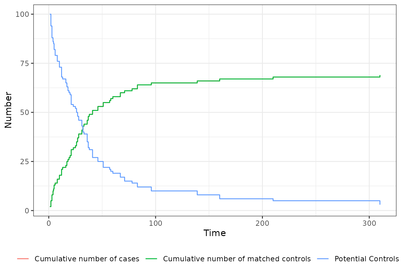

In addition to the cumulative number of cases over time and the cumulative number of matched controls over time, it also includes the number of potential controls that would have been available at $t$ . Note that if you use the inclusion argument, this number might not be non-increasing over time. Here we can see that the majority of the matching was done in the first 100 time units. Only few individuals were matched later. We can also see that the number of cases and controls is exactly the same over the entire time, which means that we always found a control for a case (remember that we used 1:1 matching here).

Next, we may also create a flowchart to describe the matching process more succintly. This can also be done easily, using the plot_flowchart() function:

plot_flowchart(m_out)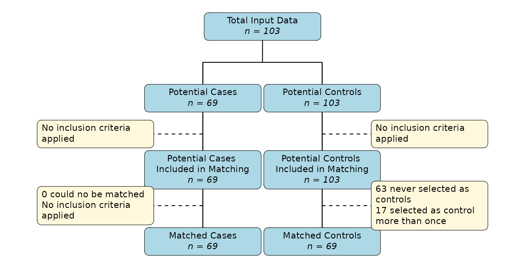

In this case, we started with the full set of 103 individuals. All of them received the transplant after $t = 0$ , so they could have theoretically been used as a control at some point in time (e.g. they are “potential controls”). Only 69 of these individuals ever received the transplant, meaning we had 69 potential cases that we could try to match. Since we did not define any inclusion criteria, there was no further subsetting here. The algorithm was able to match a control to all of these individuals. We therefore end up with 69 cases and 69 matched controls. Note that in this case, because we set replace_over_t=TRUE, 17 individuals were selected as control more than once, while 63 individuals were never selected. If we had set replace_over_t=FALSE, some individuals would not have gotten a control, because of the different lenghts of follow-up time.

We can further visualize the exact time-intervals included for each person by using the plot_timeline() function. Below we show the included time-lines for the first 7 individuals who were selected into the matching process.

plot_timeline(m_out, include=c(1, 2, 3, 4, 5, 6, 7),
              id_type="id")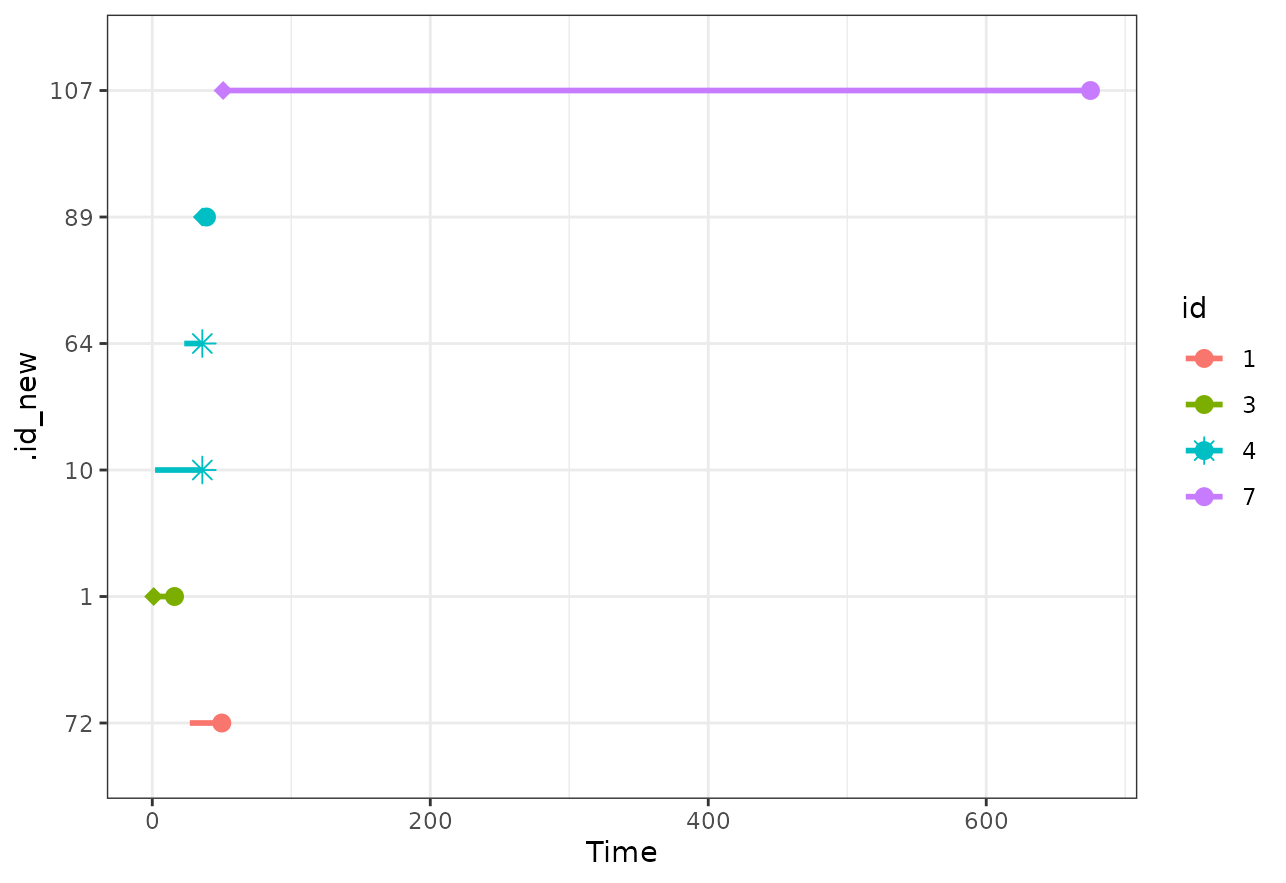

Here we can see that individuals with id %in% c(2, 5, 6) were never selected, whereas id = 4 was selected as control twice and included as a case (for a very short amount of time).

Inspecting Covariate Balance

If we rely solely on the matching process to achieve the covariate balance at baseline (e.g. we do not plan any further covariate adjustments), it is crucial to inspect whether this covariate balance between the groups was actually achieved. A first look can be gained using the summary.match_time() method:

summary(m_out)

## Call:
## match_time(formula = transplant ~ age + surgery, data = heart, 
##     id = "id", outcomes = "event", method = "brsm", replace_over_t = TRUE, 
##     match_method = "nearest")
## 
## Summary of Balance for Matched Data at Baseline:
##         Means Treated Means Control Std. Mean Diff. Var. Ratio  eCDF Mean
## age        -1.9667292    -3.0001686      0.11643458  0.7293539 0.02242926
## year        3.5988850     3.5364700      0.03530218  0.9351385 0.02601711
## surgery     0.1884058     0.1449275      0.11118740         NA 0.04347826
##           eCDF Max
## age     0.07246377
## year    0.08695652
## surgery 0.04347826
## 
## Sample Sizes:
##           Controls Treated All
## Matched         69      69 138
## Unmatched       19       0  19
## Included       103      69 103
## Supplied       103      69 103
## 
## Points in Time:
## Matching was performed at 43 unique points in time between 1 and 310.

We could also use the excellent cobalt package to obtain similar statistics in a more organized fashion:

bal.tab(m_out, stats=c("mean.diffs", "variance.ratios",
                       "ks.statistics", "ovl.coefficients"))

## Balance Measures
##            Type Diff.Un V.Ratio.Un  KS.Un OVL.Un
## age     Contin.  0.1164     0.7294 0.0725 0.0465
## year    Contin.  0.0353     0.9351 0.0870 0.0269
## surgery  Binary  0.0435          . 0.0435 0.0435
## 
## Sample sizes
##     FALSE TRUE
## All    69   69

Or present the results in form of a love.plot():

love.plot(m_out)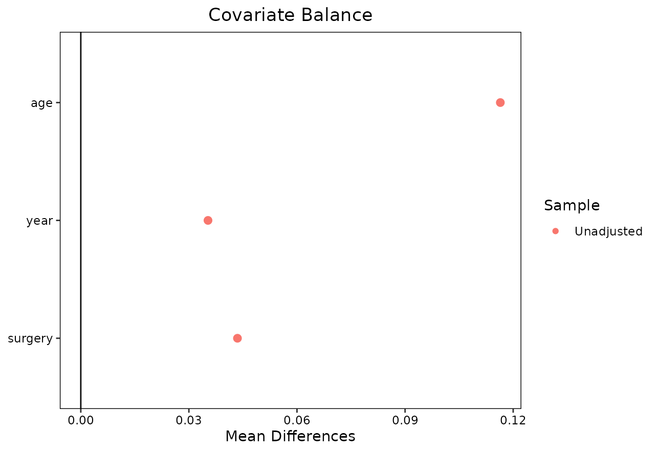

Note that both bal.tab() and love.plot() only show the balance statistics for the adjusted data here. This is in contrast to how these functions work when used on regular matchit objects created using MatchIt::matchit(). The reason for this discrepancy is, that without the time-dependent matching there is no “baseline” or other natural point in time to use in order to get values for an “unadjusted” covariate balance. This is not an issue though, since we are usually only interested in judging whether the covariate balance is sufficient after adjustment anyways. In this particular case, the covariate balance seems fine.

Analyzing Matched Data

The m_out$data object of our previously created match_time object already constitutes an almost finished dataset that might be tempting to use for further analysis. In many cases this is not a problem. It is, however, safer and thereby recommended to use the get_match_data() function instead to get the output data:

m_data <- get_match_data(m_out)

This is similar to the get_matches() or match_data() functions from the MatchIt package (although using a different name to avoid name conflicts). It automatically removes all unmatched individuals and returns the entire dataset as needed for further analysis. The first few rows of the output look like this:

head(m_data)

## Key: <id>
##       id .id_new .id_pair .treat .treat_time .next_treat_time .weights
##    <num>   <int>   <char> <lgcl>       <num>            <num>    <num>
## 1:     1      72       36  FALSE          27               NA        1
## 2:     3       1        1   TRUE           1               NA        1
## 3:     4      10        5  FALSE           2               36        1
## 4:     4      64       32  FALSE          23               36        1
## 5:     4      89       45   TRUE          36               NA        1
## 6:     7     107       54   TRUE          51               NA        1
##           age      year surgery event_status event_time
##         <num>     <num>   <num>       <lgcl>      <num>
## 1: -17.155373 0.1232033       0         TRUE         23
## 2:   6.297057 0.2655715       0         TRUE         15
## 3:  -7.737166 0.4900753       0        FALSE         34
## 4:  -7.737166 0.4900753       0        FALSE         13
## 5:  -7.737166 0.4900753       0         TRUE          3
## 6:   2.869268 0.7802875       0         TRUE        624

A detailed description about the contents of each column is given in the ?match_time documentation page. This final dataset may now be analyzed using standard analysis techniques for time-to-event endpoints. For example, we could plot standard Kaplan-Meier curves:

plot(survfit(Surv(event_time, event_status) ~ .treat, data=m_data))

A similarly popular alternative would be a Cox proportional hazards model:

mod <- coxph(Surv(event_time, event_status) ~ .treat + strata(.treat_time), data=m_data)
summary(mod)

## Call:
## coxph(formula = Surv(event_time, event_status) ~ .treat + strata(.treat_time), 
##     data = m_data)
## 
##   n= 138, number of events= 67 
## 
##               coef exp(coef) se(coef)      z Pr(>|z|)
## .treatTRUE -0.1755    0.8390   0.3398 -0.517    0.605
## 
##            exp(coef) exp(-coef) lower .95 upper .95
## .treatTRUE     0.839      1.192     0.431     1.633
## 
## Concordance= 0.543  (se = 0.069 )
## Likelihood ratio test= 0.27  on 1 df,   p=0.6
## Wald test            = 0.27  on 1 df,   p=0.6
## Score (logrank) test = 0.27  on 1 df,   p=0.6

Here we can see a hazard ratio that is smaller than 1, indicating a slight protective effect of the transplantation on the event probability, although this hazard ratio of course has a rather large confidence interval.

Going Further

This vignette is only meant to give a brief overview of the workflow and capabilities of the package. It therefore deliberately left out some important considerations, such as the target estimand, censoring schemes and caveats when analyzing the data. It also only showcases one kind of time-dependent matching. Please consult the documentation and the other vignettes of this package for further information.

Literature

Thomas, Laine E., Siyun Yang, Daniel Wojdyla, and Douglas E. Schaubel (2020). “Matching with Time-Dependent Treatments: A Review and Look Forward”. In: Statistics in Medicine 39, pp. 2350-2370.

Li, Yunfei Pail, Kathleen J. Propert, and Paul R. Rosenbaum (2001). “Balanced Risk Set Matching”. In: Journal of the American Statistical Association 96.455, pp. 870-882.

Lu, Bo (2005). “Propensity Score Matching with Time-Dependent Covariates”. In: Biometrics 61.3, pp. 721-728.

Hansen, Ben B. (2008). “The Prognostic Analogue of the Propensity Score”. In: Biometrika 95.2, pp. 481-488.

He, Kevin, Yun Li, Panduranga S. Rao, Randall S. Sung, and Douglas E. Schaubel (2020). “Prognostic Score Matching Methods for Estimating the Average Effect of a Non-Reversible Binary Time-Dependent Treatment on the Survival Function”. In: Lifetime Data Analysis 26, pp. 451-470.

Gran, Jon Michael, Kjetil Røysland, Marcel Wolbers, Vanessa Didelez, Jonathan A. C. Sterne, Bruno Ledergerber, Hansjakob Furrer, Viktor von Wyl, and Odd O. Aalen (2010). “A Sequential Cox Approach for Estimating the Causal Effect of Treatment in the Presence of Time-Dependent Confounding Applied to Data from the Swiss HIV Cohort Study”. In: Statistics in Medicine 29, pp. 2757-2768.

Ho, Daniel, Kosuke Imai, Gary King and Elizabeth A. Stuart (2011). “MatchIt: Nonparametric Preprocessing for Parametric Causal Inference”. In: Journal of Statistical Software 42.8.

Crowley, John and Marie Hu (1977). “Covariance Analysis of Heart Transplant Survival Data”. In: Journal of the American Statistical Association 72.357, pp. 27-36.

Robin Denz