The Symmetric Pair Matching Design in R

Robin Denz

Introduction

In this small vignette, we introduce the SPMD package, which can be used to apply the Symmetric Pair Matching Design, introduced by Denz et al. (2026). In a nutshell, it is a type of self-controlled method that automatically adjusts for all types of time-invariant confounders, while also automatically controlling for any confounding effects that arise through time itself. It is similar to the self-controlled case series (SCCS) design (Farrington 1995), but, contrary to the SCCS design, it does not require the user to model time trends. The SPMD package is a full implementation of the method, including multiple ways to create the required matches, confidence interval estimation and convenient plotting methods.

The package is currently not available on CRAN, but may be installed using the remotes package:

remotes::install_github("RobinDenz1/SPMD")

We load some packages here, although not all of them are required for usage of SPMD. Some are only needed for the specific contents of this vignette.

library(SPMD)
library(data.table)
library(ggplot2)
library(lme4)

What is the Symmetric Pair Matching Design?

In the following we give a very informal and short introduction to the SPM design. We highly encourage readers and users of the method to read the associated paper instead (Denz et al. 2026), which describes the method and its associated assumptions in much more detail. The goal of the SPM design is to estimate the causal relative risk of a binary time-dependent exposure on a possibly re-current binary time-to-event outcome. A classic example would be the effect of a Covid-19 vaccination on the occurrence of acute myocarditis in a short period (for example 24 days) after vaccination. Importantly, the exposure is assumed to be transient, e.g. it is assumed that it only has an effect on the outcome for a known duration after exposure, after which the risk goes back to the persons baseline level.

Under the assumption that there are no time-dependent confounders of the relationship between vaccination and the development of acute myocarditis, two potential sources of confounding remain: (1) time-invariant confounders, such as sex or genetics and (2) time itself. The latter my arise when the probability for vaccination is time-dependent and the probability for the outcome is also time-dependent, irrespective of individual characteristics. In vaccine-safety studies, this is frequently the case, especially for seasonal vaccinations such as influenza vaccines. Briefly, the method adjusts for both types of confounding through a special pair matching structure, as its name suggests.

Individuals with exposures are matched to each other, so that they can be used as control during the exposure period of the matched individual. For example, suppose there are two individuals, one vaccinated on day 50 and one vaccinated on day 120. We assume a risk period of 40 days. The resulting pairing of these two individuals would look like this:

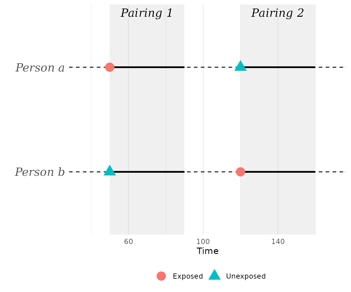
At $t = 50$, person $b$ is exposed and his risk period of length 40 begins. Since person $a$ is unexposed at this time, we can use the same duration as a control for person $b$. We then do the exact same thing at $t = 120$, when person $a$ is exposed. In a table, we would write down this pair as:

individual	time	exposure	index
a	50	0	a1
b	50	1	b1
b	120	0	b2
a	120	1	a2

It can be shown mathematically that under fairly weak assumptions of multiplicative effects, the following equation holds for each individual pairing:

$$\theta = \frac{1}{2}\log\left(\frac{\lambda_{b1} \lambda_{a2}}{\lambda_{a1} \lambda_{b2}}\right).$$

where $\lambda$ are the rate parameters of Poisson distributions that describe the number of events in the 40 day risk period in each “group”. Of course, we cannot directly calculate this value, because those rates are unknown. We do, however, observe the event counts in those times, which is enough to define estimators. Those are described further down in this vignette, after we have introduced the required data and pair matching algorithms.

Required Data

In principal, we only need information on two variables to apply the symmetric pair matching design: the exposure status and the outcome. Additionally, we need to know exactly when the exposures and outcome events occurred and for whom. The most flexible and standard way to encode this information usually used in time-to-event analysis is the start-stop or counting process format. This corresponds to the data format used to fit coxph() models (see the famous survival package) and is required by the SPMD package as well.

To give an example, we will use the sim_example_data() function of this package:

set.seed(1234)

data <- sim_example_data(n=500)
head(data)
#> Key: <.id, start>
#>      .id start  stop          X      A      Y
#>    <int> <num> <num>      <num> <lgcl> <lgcl>
#> 1:     1     0   249 -1.2070657  FALSE  FALSE
#> 2:     1   249   289 -1.2070657   TRUE  FALSE
#> 3:     1   289  1000 -1.2070657  FALSE  FALSE
#> 4:     2     0   221  0.2774292  FALSE  FALSE
#> 5:     2   221   261  0.2774292   TRUE  FALSE
#> 6:     2   261   623  0.2774292  FALSE   TRUE

This function internally uses the simDAG package to simulate this data (Denz & Timmesfeld 2026). Here, each person is identified by a unique person identifier contained in the .id column. A person may have multiple rows, where each row corresponds to a period of time (defined by the start and stop columns) in which no variables changed for that individual. For example, the first row of this dataset shows that from 0 to 249, individual with .id = 1 was unexposed (exposure is denoted by column A) and had no event (the outcome is shown in column Y). Exactly at $t = 249$, the same person is then exposed for the first time and stays exposed until $t = 289$. In other words, the exposure, and potentially other covariates, are coded so that the intervals are left-closed or right-open, often denoted using [).

The outcome events should be coded slightly differently. Events are assumed to happen exactly at the time denoted by stop. For example, individual .id = 2 experienced an event at exactly $t = 623$ in this example dataset. This data format has two main advantages. First, it allows usage of continuous time. Secondly, it is much more memory efficient than the full long-format, because we usually have to store way less rows directly. To create such datasets, the tmerge() function of the survival package, or the merge_start_stop() function from the MatchTime package (see https://robindenz1.github.io/MatchTime/) may be used.

General Syntax

Once such a dataset exists, it is very easy to apply the symmetric pair matching design. We simply need to call the sym_pair_matching() function on it, which can be done like this:

out <- sym_pair_matching(Surv(start, stop, Y) ~ A, data=data, id=".id",
                         pairs="all", estimator="moments", risk_period=30)

The function uses the classic time-to-event formula interface, in which the Surv() function is used to define the beginning (start) and end (stop) of the time intervals, as well as the outcome (Y) in this order. The right-hand side of the formula should only contain the exposure (A). In real applications, users are of course free to use any other names. Additionally, we have to specify the unique person identifier (id), the data in which we find all of these columns, the duration of the risk period after exposure (risk_period), as well as the method to generate the matched pairs (pairs) and which estimator to use (estimator). Most of these arguments are discussed in greater detail below.

Once we have created an SPMD object using this function, we can show the results using the associated summary() method:

summary(out)
#> Symmetric Pair Matching using an estimating equation based estimator
#>   Formula: Surv(start, stop, Y) ~ A 
#>   Risk period: 30 
#> 
#>   No. individuals in data = 500 
#>   No. exposed individuals = 339 
#>   No. unique exposure times = 339 
#>   No. exposed individuals with event(s) = 339 
#>   51233 symmetric pairs were created
#>   94.21% of the included observation time was used
#> 
#> Final estimate: 2.343 
#> 
#> Estimated using: exp(0.5 * log(225/41))

Creating the Matched Pairs

The sym_pair_matching() function implements different options to create the matched pairs. In the following, we give an overview of these options and show how to use them.

One unique Pairing

The first option to create pairs is to use each person / exposure period in exactly one pairing. For example, if each person has only a single exposure time, that person would be part of exactly one matched pair. This can be done in sym_pair_matching() by using pairs="one" like this:

out <- sym_pair_matching(Surv(start, stop, Y) ~ A, data=data, id=".id",
                         pairs="one", estimator="none", risk_period=30)

Here, we set estimator="none" to skip any actual estimation for now. The function then only generates the matched pairs, which can be inspected directly using:

head(out$d_matches)
#> Key: <.id_pair, .group>
#>      .id .time .max_t .id_pair     .A .group .end_time .n_events
#>    <int> <num>  <num>    <int> <lgcl>  <num>     <num>     <int>
#> 1:     3    12   1000        1  FALSE      1        42         0
#> 2:   114    12   1000        1   TRUE      2        42         0
#> 3:   114   249   1000        1  FALSE      3       279         0
#> 4:     3   249   1000        1   TRUE      4       279         0
#> 5:   319    12   1000        2  FALSE      1        42         0
#> 6:   493    12   1000        2   TRUE      2        42         0

We can also inspect the used times of the matches visually, using the associated plot() method:

plot(out)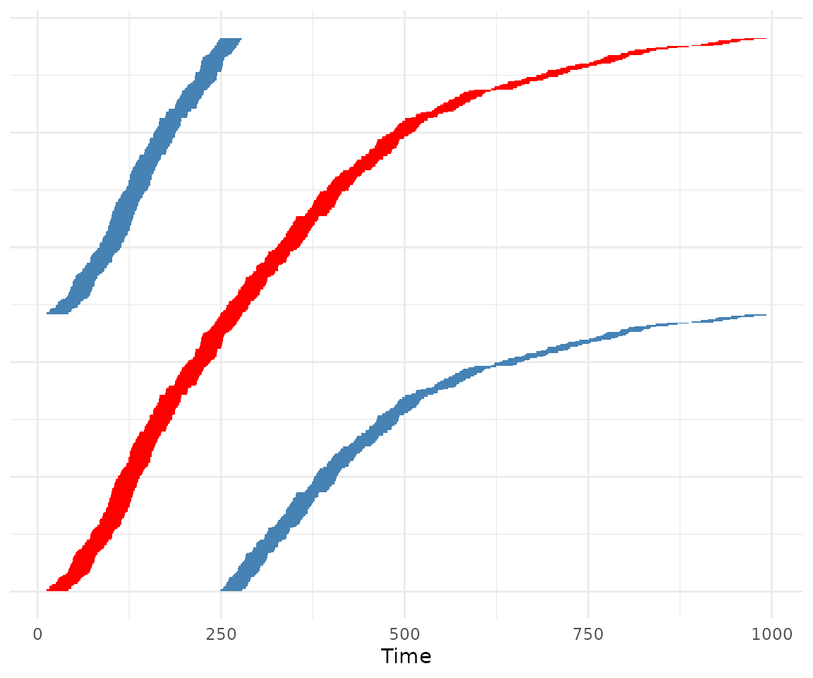

In this plot, each individual that was included in the pair-generation process forms one line of the plot (the y-axis). The red segments denote time under exposure. Blue segments denote time without exposure, that was used at some point as control in a matched pair. White segments denote observation time that remained unused.

Internally, the dataset of all individual / exposure combinations is first ordered by exposure time. Then, the dataset is “cut in half”. The first person / exposure combination (e.g. row in the dataset) of the first half is then matched to the first row of the second dataset. This is not guaranteed to work. Under some extreme distributions of exposure times, this may fail, making it a little less robust than other methods. Additionally, since we only use each exposure instance in one pair, we throw out a lot of information that we could include using the other methods. Therefore, this method is generally discouraged.

All Possible Pairs

The most statistically efficient variant is to simply use all pairs that could possible be formed. This can be done using pairs="all" instead:

out <- sym_pair_matching(Surv(start, stop, Y) ~ A, data=data, id=".id",
                         pairs="all", estimator="none", risk_period=30)

If we use plot(), we can directly see that a lot more of the observation time per person is used in the matched dataset:

plot(out)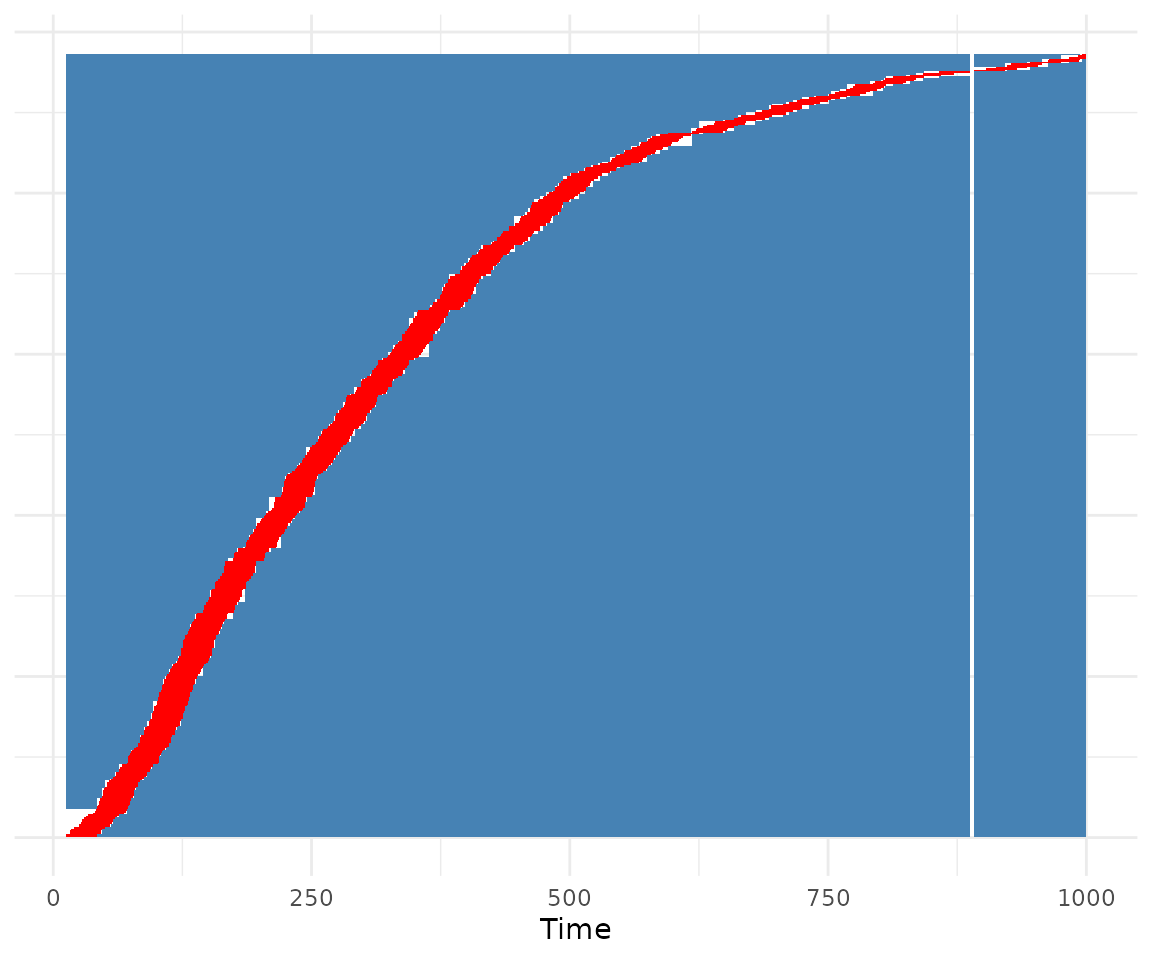

Note that even though all possible matches were generated, the plot still includes some white areas. These are observation times that could not be used in any of the possible matches. Although using all possible matches is statistically very efficient, it is very heavy computationally. The upper limit of possible matches grows very fast and can be calculated as

$$\frac{n \cdot (n-1)}{2},$$

where $n$ is the number of unique individual / exposure instances. Due to this fast growth, it might not even be possible computationally to generate all pairs with large $n$. Luckily, we do not actually need to do this. It is perfectly acceptable to use a fixed large number of randomly chosen pairs instead.

Fast random selection

The package implements a random selection of pairs in two ways. The first one is a fast selection algorithm, which generates all possible pairs first and then takes a random sample of size n_pairs from the resulting dataset. This can be done using pairs="random2":

out <- sym_pair_matching(Surv(start, stop, Y) ~ A, data=data, id=".id",
                         pairs="random2", estimator="none", risk_period=30,
                         n_pairs=100000)

Here we used a 100,000 matched pairs, as specified through the n_pairs argument. If we run plot() on this again, we can see that we are still using quite a lot of the observed time per person at least once:

plot(out)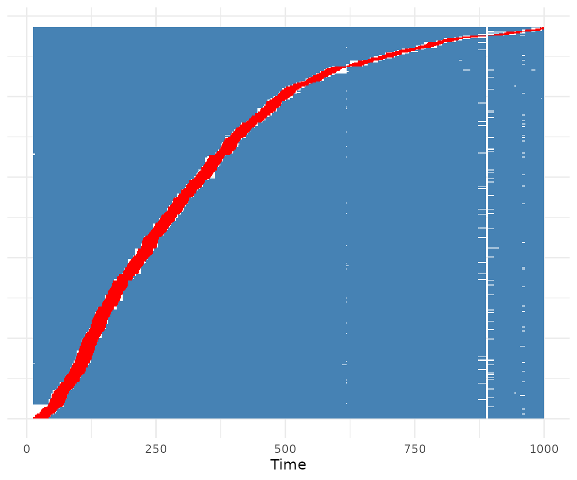

This may work for fairly large datasets and it is fairly fast, but eventually it will fail as well due to the required RAM of the first step. If it fails, we may use pairs="random1" instead.

Memory efficient random selection

To circumvent the problem of having to create all possible matches first, we may use an iterative algorithm instead. Here, we randomly sample batch_size / 2 rows from the individual / exposure dataset and match them to further, also randomly sampled, batch_size / 2 rows. We then remove duplicates and invalid matches. All generated matches are then added to the output. If we have created n_pairs matches, we stop. If we have not, we repeat the process until we found enough matches or until rand_max_iter iterations were executed. This can be done using pairs="random1":

out <- sym_pair_matching(Surv(start, stop, Y) ~ A, data=data, id=".id",
                         pairs="random1", estimator="none", risk_period=30,
                         n_pairs=100000)

It is often quite a bit slower than pairs="random2", because of its iterative nature and the sometimes large amount of invalid or repeated matches created during the iterations. The main advantage is that it can always be used, regardless of how many matches are possible.

Which pair generation method should I use?

The amount of options naturally raises the question, which option is the best. Whenever using estimator="moments" (which should be used in most cases), we recommend trying pairs="all" first, because it is the statistically most efficient option. If this fails due to the amount of matches being too large, it is best to try pairs="random2" next, with a large number of n_pairs such as 1,000,000. If that still fails due to RAM issues, pairs="random1" is the best alternative (again with a large value for n_pairs). One-to-one matching as implemented in pairs="one" should generally only be used if the dataset is gigantic, or when using estimator="glmm".

Estimators

After having created the symmetric pair matches, we still have to apply an estimator to obtain the relative risk of interest. The package implements two main estimators, the main empirical moments based estimator (estimator="moments") and an experimental estimator based on a generalized linear mixed Poisson model (estimator="glmm").

Empirical moments based estimator

Given $m$ pairs of individuals, the estimator is defined as:

$$\hat{\theta}_m = \frac{1}{2} \ln\! \left(\frac{\frac{1}{m}\sum_{i = 1}^m X_{b1} X_{a2}}{\frac{1}{m}\sum_{i = 1}^m X_{a1} X_{b2}}\right),$$

where $X_{a1}$, $X_{a2}$, $X_{b1}$ and $X_{b2}$ denote the observed event counts in each “index” inside a pair. Essentially, we average over individual level products of events in both the denominator and numerator. By taking exp() of the resulting $\hat{\theta}_m$, we obtain an estimate of the causal risk ratio. In this package, this estimator can be used by setting estimator="moments".

Generalized linear mixed model based estimator

An alternative experimental estimator is based on a generalized linear mixed Poisson model, where an individual and time-specific random effect is modeled directly. This method may be more efficient than the moments based estimator, because it utilizes information across pairs more efficiently, but it is also fairly difficult to fit. In many cases, it will not converge in practice. We recommend not using this estimator for now, as its theoretical properties have not been studied in detail.

Confidence interval estimation

The estimators by themselves only return a point estimate (e.g. an estimate of the relative risk). In most applications, we are, however, also interested in estimating the uncertainty of this point estimate. This is often done using confidence intervals. We may also wish to test the hypothesis, that the true relative risk is 1, which is often done using p-values. Currently, no equation exists that could be used to directly estimate the standard error of the estimate, which would be required for both applications. We therefore usually rely on bootstrapping, which is implemented into the sym_pair_matching() function through the bootstrap argument:

out <- sym_pair_matching(Surv(start, stop, Y) ~ A, data=data, id=".id",
                         pairs="all", estimator="moments", risk_period=30,
                         bootstrap=TRUE, n_boot=1000)
summary(out)
#> Symmetric Pair Matching using an estimating equation based estimator
#>   Formula: Surv(start, stop, Y) ~ A 
#>   Risk period: 30 
#> 
#>   No. individuals in data = 500 
#>   No. exposed individuals = 339 
#>   No. unique exposure times = 339 
#>   No. exposed individuals with event(s) = 339 
#>   51233 symmetric pairs were created
#>   94.21% of the included observation time was used
#> 
#> Final estimate: 2.343 
#> 95% CI: [1.356; 3.855]
#> P-Value: 0.006 
#> 
#> Estimated using: exp(0.5 * log(225/41))
#> Bootstrap CI based on 1000 bootstrap replications

Here, we first draw n_boot random samples with replacement from all individuals, where the size of the samples is equal to the number of unique individuals in the dataset. Then, we apply the pair matching to each of these datasets. Afterwards, we apply the estimator to all matched datasets. The result is a vector of n_boot bootstrap estimates. To estimate a 95% confidence interval, we use the percentile method, in which the lower 0.025 and upper 0.975 quantiles of this bootstrap distribution is used directly. P-values are calculated similarly, although with the caveat that a bootstrap p-value can never be smaller than 1 / n_boot.

We can inspect the distribution of the bootstrap samples directly using something like:

plot(density(out$boot_est))

Ideally, the distribution should look more or less Gaussian. In any case, it is recommended to set the number of bootstrap samples high enough so that the distribution looks fairly smooth. n_boot=1000 is a good start, but may not always be sufficient.

Bootstrapping may become fairly computationally expensive, particularly with large samples and pairs="all" or pairs="random1" / pairs="random2" when using many matches. We have implemented some computational tricks that keep the computation time low, particularly when using pairs="all". In this case, the pair matching is only done once and the bootstrap samples are generated directly from all pairs through re-weighting them. This is possible because repeated inclusion of individuals never generates new samples (individuals cannot match themselves, because the risk periods would overlap). Additionally, the n_cores argument may be used to run the bootstrap calculations on multiple processing cores, potentially saving much more time as well.

Some subtleties

Censoring

Right-censoring is directly supported by this package. The underlying algorithm uses pairs in which no observation period is censored, and pairs in which the right-censoring occurs after the larger of the two exposure times in a pair. In the latter case, both individuals inside the pair are censored at the minimum censoring time when calculating $X_{a2}$ and $X_{b2}$. This way, the time effects still cancel out. For more information and required assumptions regarding censoring, please consult the associated paper (Denz et al. 202X).

Bounds of the risk period

The bounds argument allows users to specify whether / which endpoints of the risk periods defined by the exposure times and risk_period arguments should be included or excluded. It is particularly important to specify this argument if the measurements of exposure and outcome times is done in discrete time. See ?sym_pair_matching for a full explanations on supported values.

Time zero

In randomized controlled trials, time zero (e.g. the begin of the observation period) is well defined for each participant in the study. This is not necessarily the case for retrospective studies. For example, when analyzing electronic health records based data, multiple choices for time zero, such as the date of a diagnosis or the first date of eligibility, may be appropriate. Theoretically, any time scale may be used for the application of SPMD. It is, however, crucial that the choice of time scale reflects the time trends the user wants to adjust for. For example, if time trends in the outcome are caused by calender time and are shared across individuals, the time scale should be the calender time. If, on the other hand, the time trends are anchored to time since a diagnosis, than time zero should be the date of diagnosis.

References

Denz, Robin, Filippo Saatkamp, Katharina Meiszl and Nina Timmesfeld (2026). “The Symmetric Pair Matching Design: A Self-Controlled Method with Automatic Adjustment for Time Effects”. arXiv Preprint. doi: 10.48550/arXiv.2608.25979.

Farrington, C. Paddy (1995). “Relative Incidence Estimation from Case Series for Vaccine Safety Evaluation”. In: Biometrics 51.1, pp. 228–235. doi: 10.2307/2533328.

Denz, Robin and Nina Timmesfeld (2026). “Simulating Complex Cross-Sectional and Longitudinal Data using the simDAG R Package”. Journal of Statistical Software 116 (2), doi: 10.18637/jss.v116.i02.