Plot Confounder-Adjusted Cumulative Incidence Functions

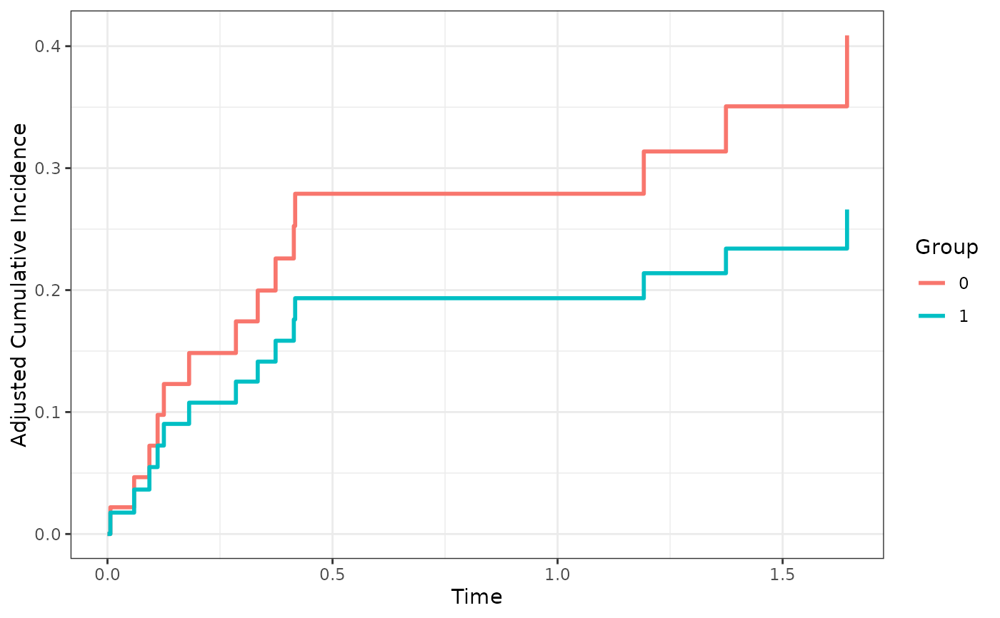
A function to graphically display confounder-adjusted cumulative incidence functions which where previously estimated using the adjustedcif function. The user can customize the plot using a variety of options. Internally it uses the ggplot2 package, so additional not implemented features can be added using the standard ggplot2 syntax. This function also includes the option to use isotonic regression on the CIFs, which is of benefit if the estimated curves are not monotone.

Usage

# S3 method for class 'adjustedcif'
plot(x, conf_int=FALSE, max_t=Inf,
     iso_reg=FALSE, force_bounds=FALSE,
     use_boot=FALSE, color=TRUE,
     linetype=FALSE, facet=FALSE,
     line_size=1, line_alpha=1, xlab="Time",
     ylab="Adjusted Cumulative Incidence",
     title=NULL, subtitle=NULL, legend.title="Group",
     legend.position="right",
     gg_theme=ggplot2::theme_classic(),
     ylim=NULL, custom_colors=NULL,
     custom_linetypes=NULL,
     single_color=NULL, single_linetype=NULL,
     conf_int_alpha=0.4, steps=TRUE,
     censoring_ind="none",
     censoring_ind_size=0.5,
     censoring_ind_alpha=1,
     censoring_ind_shape=17,
     censoring_ind_width=NULL,
     ...)

Arguments

x

An adjustedcif object created using the adjustedcif function.

conf_int

A logical variable indicating whether the confidence intervals should be drawn.

max_t

A number indicating the latest event time which is to be plotted.

iso_reg

A logical variable indicating whether the estimates should be monotonized using isotonic regression. See details.

force_bounds

A logical variable indicating whether the 0 and 1 bounds of the CIFs should be forced in the plot. See details.

use_boot

A logical variable denoting whether the bootstrapped estimates should be used for the curves and their confidence intervals. Can only be used if they were calculated. See adjustedcif.

color

A logical variable indicating whether the curves should be colored differently. The custom_colors argument can be used to directly specify which colors to use. Alternatively the single_color argument can be used if everything should have the same color.

linetype

A logical variable indicating whether the curves should have different linetypes. The custom_linetypes argument can be used to directly specify which linetypes to use. Alternatively the single_linetype argument can be used if all curves should have the same linetype.

facet

A logical variable indicating whether the curves should be in different facets.

line_size

A number controlling the thickness of the curves.

line_alpha

A number controlling the transparency level of the curves.

xlab

A character string to be used as the X-Axis label of the plot.

ylab

A character string to be used as the Y-Axis label of the plot.

title

A character string to be used as the title of the plot. Set to NULL (default) if no title should be used.

subtitle

A character string to be used as the subtitle of the plot. Set to NULL (default) if no subtitle should be used.

legend.title

A character string to be used as the title of the legend. Set to NULL if no legend should be included.

legend.position

A character string specifying the position of the legend. Ignored if legend_title=NULL.

gg_theme

A ggplot2 theme object which will be used for the plot.

ylim

A numeric vector of length two, specifying the limits of the Y-Axis. Set to NULL to use the ggplot2 default values.

custom_colors

A (named) vector to specify the colors of each CIF and possibly its confidence region. Set to NULL to use the ggplot2 default values. Ignored if color=FALSE.

custom_linetypes

A (named) vector to specify the linetype of each CIF. Set to NULL to use the ggplot2 default values. Ignored if linetype=FALSE.

single_color

A single color to use for every curve, irrespective of group status. If color is specified as well this argument will override it, but also generate a warning. Set to NULL (default) to ignore this argument.

single_linetype

A single linetype to use for every curve, irrespective of group status. If linetype is specified as well this argument will override it, but also generate a warning. Set to NULL (default) to ignore this argument.

conf_int_alpha

A number indicating the level of transparency that should be used when drawing the confidence regions.

steps

A logical variable indicating whether the CIFs should be plotted as a step function or using straight lines. Straight lines should not be used with a simple Aalen-Joahnsen estimator. It is recommended to only use straight lines when a sufficiently fine grid of time points was used in the estimation step.

censoring_ind

What kind of indicator to plot for censored observations on the CIFs. Must be one of "none" (plotting no indicators at all, the default), "lines" (plotting small vertical lines) and "points" (plotting points). Those will be affected by linetype and color as well. Observations who failed due to a competing event are not considered as censored here.

censoring_ind_size

A numeric value specifying the size of the censoring indicators. Ignored if censoring_ind="none".

censoring_ind_alpha

A numeric value specifying the alpha level of the censoring indicators. Ignored if censoring_ind="none".

censoring_ind_shape

A numeric value specifying the shape of the censoring indicators when using censoring_ind="points". Ignored otherwise. For available shapes see ?geom_point.

censoring_ind_width

A numeric value specifying the width of the censoring indicators. Ignored unless censoring_ind="lines". By default (censoring_ind_width=NULL) the width of the censoring indicators is equal to 5 percent of the plot height.

...

Currently not used.

Details

When using certain methods there is no guarantee that the resulting estimated CIFs are monotonically increasing. This is unfortunate since we know that it has to be the case. Isotonic regression can be used to fix this problem by ensuring that the CIFs are actually monotonically increasing everywhere, while also being as close to the observations as possible. Westling et al. (2020) showed mathematically that this usually does not add any systematic bias to the estimates. More information on the method can be found in Robertson et al. (1988). This adjustment can be done using this function by setting iso_reg to TRUE.

Similarly, some methods can produce estimates that lie outside the theoretical 0 and 1 bounds of probability. By setting force_bounds to TRUE these estimates are manually set to either 0 or 1 (whichever is closer).

Value

Returns a ggplot2 object.

References

Ted Westling, Mark J. van der Laan, and Marco Carone (2020). "Correcting an Estimator of a Multivariate Monotone Function with Isotonic Regression". In: Electronic Journal of Statistics 14, pp. 3032-3069

Tim Robertson, F. T. Wright, and R. L. Dykstra (1988). Order Restricted Statistical Inference. Hoboken: John Wiley & Sons

Author

Robin Denz

See also

adjustedcif, ggplot, geom_stepribbon, isoreg

Examples

library(adjustedCurves)
library(survival)

if (requireNamespace("riskRegression") & requireNamespace("prodlim") &
    requireNamespace("ggplot2")) {

library(riskRegression)
library(prodlim)
library(ggplot2)

set.seed(42)

# simulate some data as example
sim_dat <- sim_confounded_crisk(n=50)
sim_dat$group <- as.factor(sim_dat$group)

# calculate a Cause-Specific-Cox model
cox_mod <- CSC(Hist(time, event) ~ x1 + x3 + x5 + group,
               data=sim_dat)

# use it to calculate adjusted CIFs with bootstrapping (for cause = 1)
adjcif <- adjustedcif(data=sim_dat,
                      variable="group",
                      ev_time="time",
                      event="event",
                      method="direct",
                      outcome_model=cox_mod,
                      conf_int=TRUE,
                      bootstrap=TRUE,
                      n_boot=15, # should be much bigger in reality
                      cause=1)

# plot the curves with default values
plot(adjcif)

# plot after applying isotonic regression
plot(adjcif, iso_reg=TRUE)

# plot with confidence intervals estimated using asymptotic variances
plot(adjcif, conf_int=TRUE)

# plot with confidence intervals estimated using bootstrapping
plot(adjcif, conf_int=TRUE, use_boot=TRUE)

# plot with different linetypes only
plot(adjcif, linetype=TRUE, color=FALSE, facet=FALSE)

# plot with different facets only
plot(adjcif, linetype=FALSE, color=FALSE, facet=TRUE)

# plot with different linetypes and different colors
plot(adjcif, linetype=TRUE, color=TRUE, facet=FALSE)

# plot with some custom characteristics
plot(adjcif, legend.position="bottom", linetype=TRUE,
     custom_colors=c("green", "blue"), legend.title="Custom",
     title="Custom Plot", conf_int=TRUE, linesize=0.5)

# adding further ggplot2 elements
plot(adjcif) + theme_bw()
}
#> Warning: Rare event 
#> Warning: Estimated risk outside the range [0,1].
#> Consider setting the argument 'product.limit' to FALSE. 
#> Warning: Rare event 
#> Warning: Rare event 
#> Warning: Rare event 
#> Warning: Loglik converged before variable  1 ; coefficient may be infinite. 
#> Warning: Rare event 
#> Warning: Rare event 
#> Loading required namespace: pammtools