Simulating Data using a Discrete-Event Approach
Robin Denz
Source:vignettes/v_sim_discrete_event.Rmd
v_sim_discrete_event.RmdIntroduction
In this small vignette, we introduce the
sim_discrete_event() function, which can be used to
generate complex longitudinal data with a continuous time scale based on
the discrete-event simulation (DES) framework (Banks et al. 2014). It is very similar to the
sim_discrete_time() function in spirit, but relies on a
completely different algorithm to generate the data. This algorithm is
usually much faster than the discrete-time approach, while also being
more precise. The drawback is some added complexity and a little less
flexibility. For example, in sim_discrete_event(),
continuous, categorical or count-based time-dependent variables are
currently not supported. Only binary variables added using the
"next_time" node type may be used.
The goal of the sim_discrete_event() function is not to
provide a general framework for DES. Multiple other R packages, such as
simmer (Ucar et al. 2019; Degeling
et al. 2025) and DES (Matloff
2017), as well as software packages outside R have been developed
for that purpose and are much more useful in this regard. Instead, the
aim of this function is to provide a specific, but fairly general, DES
model that may be used to generate data from DAG based description of
the data generation process (DGP). In other words: if you want to
perform a classic DES with interacting agents using a classic simulation
modeling approach, this is probably not the right package for you. If
you want to generate complex time-dependent data based on a stochastic
model, you have come to the right place.
Throughout the vignette, we assume that the reader is already
familiar with the simDAG syntax. If this is not the case,
we recommend consulting the introductory vignette or the main paper
associated with this package first (Denz and
Timmesfeld 2026).
What is Discrete-Event Simulation and Why Use it?
In a discrete-event simulation (DES), the data is generated according
to a statistical model, which describes a system as a sequence of
distinct (or discrete) events that happen in continuous time and may
influence each other. Any DES starts with the generation of
individuals at
that have some characteristics, such as values of multiple covariates.
The full description of all individuals is considered to be the
state of the simulation here. This state only ever
changes when some event occurs. A simple example for an
event would be a variable changing its value from
FALSE to TRUE or vice versa. If such an event
occurs, the time of the simulation is advanced to the timing of this
event. The state of the simulation is then updated to reflect the
changes brought on by this event. Next, the time until the next event is
generated and the process is repeated until some condition is met. The
flowchart below gives a generalized description of a DES as considered
here.
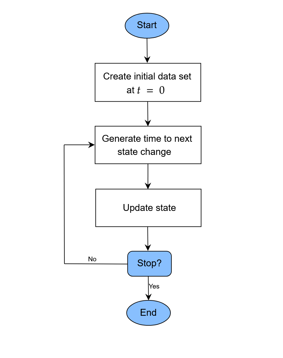
A generalized flow-chart of the discrete-event simulation approach
This approach has many names and usages in the literature. In physics
and chemistry, the particular variant discussed here is known as the
Gillespie algorithm (Gillespie 1976,
1977), or the next reaction or first reaction
method (Anderson 2007). Formally, it is a
mathematically exact method to generate random trajectories from a known
(not necessarily Markovian) stochastic process (Masuda and Rocha 2018). Formal descriptions of
the algorithm are given in the cited literature. The most general
description of the DES (or Gillespie algorithm) implemented in
sim_discrete_event() is as follows for every
individual:
- At
,
initialize the baseline covariate values and set all
time-dependent covariates to
FALSE.
- At
,
initialize the baseline covariate values and set all
time-dependent covariates to
- For each of the considered time-dependent variables, generate the time until the next change based on some distributional assumptions (possibly dependent on any variables contained in the current state)
- Advance the simulation to the minimum of the values drawn in step (2).
- Update the value of the time-dependent variable that generated this event.
- Go back to step (2) and repeat until either some condition is met or no changes are possibly anymore (may happen if every time-dependent variable has reached a terminal state).
The sim_discrete_event() directly implements this
workflow, assuming that individuals (rows in the data) do
not influence each other. A data set at
is either simulated using the sim_from_dag() function or
supplied directly by the user (using the t0_data argument).
This data set is then updated according to the time-dependent nodes
added to the dag using node_td() calls. After
each update, the state of the simulation is saved, so that the final
output is a single dataset in the start-stop format. Below we give a
short example on how this works in practice. We use a similar example to
the one used in the discrete-time simulation vignette, to allow direct
comparisons with the discrete-time approach.
Defining the DAG
As for the other simulation functions in this package, the definition
of a DAG is the first required step. Any amount of time-independent
variables specified using standard node() function calls
are supported. Time-dependent nodes should be specified using the
node_td() function instead. Importantly, for
sim_discrete_event(), only time-dependent nodes of type
"next_time" are supported. For more examples and guidance
on how to generally define a DAG, please consult the other vignettes and
documentation pages of this package.
A single time-dependent variable
For illustrative purposes, we will start with a small comparison of
the discrete-time simulation approach and the discrete-event approach.
Consider that we are interested in simulating the time until
death for
individuals. Lets ignore the influence of any other variables for the
moment and just consider death by itself. Suppose that
death has a fixed probability of 0.01 to occur during each
time-unit.
Discrete-Time approach
In a discrete-time simulation, we would simply draw Bernoulli trials
with a probability of 0.01 at
.
If the trial returns a 1, we are done and save the time. If it returns a
0, we increase
by one and repeat until we are finished. This can be done using the
sim_discrete_time() function using the following code:
library(simDAG)
library(data.table)
#>
#> Attaching package: 'data.table'
#> The following object is masked from 'package:base':
#>
#>     %notin%
library(ggplot2)

set.seed(1234)

dag_dts <- empty_dag() +
  node_td("death", type="time_to_event", prob_fun=0.01, event_duration=Inf)

simDTS <- sim_discrete_time(dag_dts, n_sim=10, max_t=10000000,
                            break_if=all(data$death_event==TRUE))
head(simDTS$data)
#>      .id death_event death_time
#>    <int>      <lgcl>      <int>
#> 1:     1        TRUE         98
#> 2:     2        TRUE         20
#> 3:     3        TRUE         13
#> 4:     4        TRUE        112
#> 5:     5        TRUE         36
#> 6:     6        TRUE         54
Here, we set the max_t argument to a very large number
and told the function to stop once everyone has died using the
break_if argument. This approach works well, but it is also
incredibly inefficient in this simple example. Since death
has a constant probability of 0.01, we could also simply sample time
values from an exponential distribution with rate=0.01.
This is exactly what will be exploited in the DES approach.
Discrete-Event approach
Since we are only interested in a single variable, which has a terminal state (once you are dead, there is no going back), we only need one time-jump and thus only one iteration in the DES approach, while we needed potentially hundreds or thousands in the discrete-time approach. The following code may be used to implement this:
dag_des <- empty_dag() +
  node_td("death", type="next_time", prob_fun=0.01, event_duration=Inf)

simDES <- sim_discrete_event(dag_des, n_sim=10, target_event="death",
                             keep_only_first=TRUE)
head(simDES)
#> Key: <.id, start>
#>      .id start       stop  death
#>    <int> <num>      <num> <lgcl>
#> 1:     1     0 102.242570   TRUE
#> 2:     2     0 140.148734   TRUE
#> 3:     3     0 104.549136   TRUE
#> 4:     4     0  91.690158   TRUE
#> 5:     5     0   1.877996   TRUE
#> 6:     6     0 147.742697   TRUE
There are some differences to the output of the
sim_discrete_time() function. First, because we are using
the DES approach, the time is continuous and not discrete. Secondly, the
output is naturally in the start-stop format, because there would be no
other useful way to represent it. Because there is only one change, each
individual only has one row in the dataset and it is thus still almost
equivalent to the output of the discrete-time approach.
In this example the sim_discrete_event() output is
exactly equal to just calling rexp(10, rate=0.01), while
the sim_discrete_time() output is a discrete-time
approximation to it.
Two interrelated time-dependent variables
We will now make the example a little more complex, by including a time-dependent variable which directly influences the probability of death. Consider the following code:
prob_death <- function(data) {
  0.001 * 0.8^(data$treatment)
}

dag <- empty_dag() +
  node_td("treatment", type="next_time", prob_fun=0.01,
          event_duration=100) +
  node_td("death", type="next_time", prob_fun=prob_death,
          event_duration=Inf)

sim <- sim_discrete_event(dag, n_sim=10, remove_if=death==TRUE,
                          target_event="death", keep_only_first=TRUE)
Here, we specified two time-dependent nodes of type
"next_time". The first one denotes the
treatment, which has a fixed probability of being given to
a person. It then has an effect for 100 time units, after which the
variable turns back to FALSE. Once it is FALSE
again, it may be given to the same person again immediately, with a
probability of 0.01. The probability of the death of a
person is now no longer fixed, but a function of the
treatment status. The general probability of death is 0.001
per time unit, but it is reduced by a factor of 0.8 if the
treatment is currently in effect.
Importantly, in this simulation we had to use one of the three
arguments that define an end of the simulation: max_t,
remove_if or break_if. We specified
remove_if, so that all individuals who die are no longer
part of the simulation. Alternatively, we could have gotten a similar
effect using the break_if argument, or limit the amount of
time the simulation may run with max_t. The latter is not
very useful here, because we are interested in the time of death. If we
hadn’t used any of these arguments, the simulation would be updated
exactly 1000 times per person (default value of the
max_iter argument), because treatment does not
have a terminal state (both its event_duration and
immunity_duration are finite). The
target_event argument is only used to make the output a
little prettier.
The generated data for the first individual look like this:
head(sim, 9)
#> Key: <.id, start>
#>      .id     start      stop treatment  death
#>    <int>     <num>     <num>    <lgcl> <lgcl>
#> 1:     1   0.00000  15.65804     FALSE  FALSE
#> 2:     1  15.65804 115.65804      TRUE  FALSE
#> 3:     1 115.65804 168.33340     FALSE  FALSE
#> 4:     1 168.33340 268.33340      TRUE  FALSE
#> 5:     1 268.33340 420.23653     FALSE  FALSE
#> 6:     1 420.23653 520.23653      TRUE  FALSE
#> 7:     1 520.23653 606.02564     FALSE  FALSE
#> 8:     1 606.02564 706.02564      TRUE  FALSE
#> 9:     1 706.02564 860.85932     FALSE   TRUE
As can be seen, the treatment keeps switching between
TRUE and FALSE until the death is
eventually reached. If we increased n_sim and fit a Cox
proportional hazards regression model with the time-to
death as the endpoint and the treatment as
covariate, we would be able to recover the 0.8 as the hazard ratio for
the treatment. The same strategy could of course be used for any amount
of time-varying variables.
Above, we used the prob_fun argument to specify the
probabilities, so that the connection to the
sim_discrete_time() approach is more clear. Alternatively,
we could also use the much more convenient formula
interface:
dag <- empty_dag() +
  node_td("treatment", type="next_time", prob_fun=0.01,
          event_duration=100) +
  node_td("death", type="next_time",
          formula= ~ log(0.001) + log(0.8)*treatment, link="log",
          event_duration=Inf)

sim <- sim_discrete_event(dag, n_sim=10, remove_if=death==TRUE,
                          target_event="death", keep_only_first=TRUE)
Here, we simply specified the log-binomial model as one would when
specifying a simple binomial regression model (see
?node_binomial). Note that although the results are
theoretically equivalent when the same seed is used, they are not
identical in practice, due to small floating point errors. This should
not be an issue in practice.
Some things to consider
Time-Dependent probabilities and effects
By default, the time until the next event is generated using a random
draw from an exponential distribution. This approach, however, assumes
that the probability of occurrence is independent of the time. We can
relax this assumption in multiple ways. The most simply way is to use
the redraw_at_t argument. This argument allows users to
specify points in time at which the time to the next event should be
re-drawn. By additionally making the probability function supplied to a
time-dependent node time-specific, we can then use a piecewise-constant
baseline event probability, instead of a truly constant one. Consider
the following code:
prob_death <- function(data) {
  base_p <- fifelse(data$.time > 300, 0.005, 0.001)
  base_p * 0.8^(data$treatment)
}

dag <- empty_dag() +
  node_td("treatment", type="next_time", prob_fun=0.01,
          event_duration=100) +
  node_td("death", type="next_time", prob_fun=prob_death,
          event_duration=Inf)

sim <- sim_discrete_event(dag, n_sim=10, remove_if=death==TRUE,
                          target_event="death", redraw_at_t=300,
                          keep_only_first=TRUE)
head(sim)
#> Key: <.id, start>
#>      .id     start      stop treatment  death
#>    <int>     <num>     <num>    <lgcl> <lgcl>
#> 1:     1   0.00000  32.13286     FALSE  FALSE
#> 2:     1  32.13286 132.13286      TRUE  FALSE
#> 3:     1 132.13286 300.00000     FALSE  FALSE
#> 4:     1 300.00000 440.08265     FALSE  FALSE
#> 5:     1 440.08265 540.08265      TRUE  FALSE
#> 6:     1 540.08265 648.71324     FALSE  FALSE
In this code, the baseline probability is 0.001 until
and then increases to 0.005. It is not sufficient to only define the
probability function this way, because then there would be no way for
the simulation itself to know that the event durations have to be
re-drawn. For example, lets say the death time drawn at
for some person is 678 and assume that treatment has no
effect for this individual. This time was generated using a rate of
0.001, so only the time until 300 is valid. At
,
we therefore have to re-draw another time from a truncated exponential
distribution with the new rate of 0.005 (truncated at 300).
The same strategy could be used to define piecewise-constant
time-dependent effects as well. One would only need to adjust the
prob_death() function so that it has a different factor for
treatment depending on the time. Using continuously
changing probabilities is also possible, but requires a different
approach. The easiest way to do this is by using the model
argument. Consider the code below:
dag <- empty_dag() +
  node_td("treatment", type="next_time", prob_fun=0.01,
          event_duration=100) +
  node_td("death", type="next_time",
          formula= ~ log(0.8)*treatment, model="cox",
          surv_dist="weibull", gamma=1.5, lambda=0.0001,
          event_duration=Inf)

sim <- sim_discrete_event(dag, n_sim=10, remove_if=death==TRUE,
                          target_event="death", keep_only_first=TRUE)
head(sim)
#> Key: <.id, start>
#>      .id     start      stop treatment  death
#>    <int>     <num>     <num>    <lgcl> <lgcl>
#> 1:     1   0.00000  40.59338     FALSE  FALSE
#> 2:     1  40.59338 140.59338      TRUE  FALSE
#> 3:     1 140.59338 171.25288     FALSE  FALSE
#> 4:     1 171.25288 271.25288      TRUE  FALSE
#> 5:     1 271.25288 314.34103     FALSE  FALSE
#> 6:     1 314.34103 414.34103      TRUE  FALSE
Here, we use a Cox proportional hazards model with a Weibull baseline
hazard function to generate the time of death instead of
directly defining the probability functions and drawing values using an
exponential distribution. Since the Weibull distribution is not constant
over time, this is a valid strategy if we want continuously changing
baseline event probabilities.
Since node_cox() (the function that is used to generate
the times following a Cox model under the hood) allows users to specify
arbitrary baseline hazard functions, users may use any kind of
time-dependent probabilities. For example, lets define this arbitrary
baseline hazard for death:
fbasehaz <- function(t) {
  0.0002 +
    0.001 * exp(-((t - 200)^2) / (2 * 50^2)) + # first hill
    0.0008 * exp(-((t - 700)^2) / (2 * 80^2))  # second hill
}
Plotted, it looks like this for the first 1000 time units:
plotdata <- data.frame(time=1:1000, val=fbasehaz(1:1000))

ggplot(plotdata, aes(x=time, y=val)) +
  geom_line() +
  theme_minimal()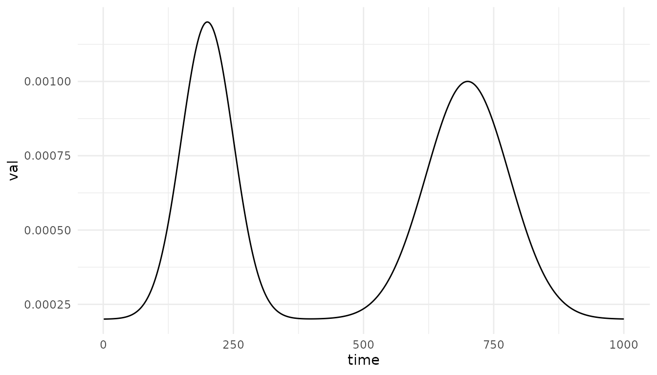
We can use this function as a baseline hazard for death
through the surv_dist argument of node_cox()
like this:
dag <- empty_dag() +
  node_td("treatment", type="next_time", prob_fun=0.01,
          event_duration=100, immunity_duration=Inf) +
  node_td("death", type="next_time",
          formula= ~ log(0.8)*treatment, model="cox",
          surv_dist=fbasehaz, basehaz_grid=1:1000000,
          event_duration=Inf, extrapolate=TRUE)

sim <- sim_discrete_event(dag, n_sim=10, remove_if=death==TRUE,
                          target_event="death", keep_only_first=TRUE,
                          max_t=10000)
head(sim)
#> Key: <.id, start>
#>      .id     start       stop treatment  death
#>    <int>     <num>      <num>    <lgcl> <lgcl>
#> 1:     1   0.00000   10.02079     FALSE  FALSE
#> 2:     1  10.02079  110.02079      TRUE  FALSE
#> 3:     1 110.02079 1487.77199     FALSE   TRUE
#> 4:     2   0.00000   60.61419     FALSE  FALSE
#> 5:     2  60.61419  160.61419      TRUE  FALSE
#> 6:     2 160.61419 4432.02708     FALSE   TRUE
Internally, the time to death is now generated by
following steps: (1) numerically calculating the cumulative baseline
hazard using the trapezoid rule over the grid of time points specified
using basehaz_grid, (2) interpolating the increments
linearly to obtain a smooth function, (3) inverting the estimated
cumulative hazard function, (4) simulating cumulative hazards from the
defined model and (5) reading off the corresponding survival time
through the inverted cumulative hazard function. Note that this method
can only generate data up to max(basehaz_grid).
In theory, the same strategy could be used for any other
time-to-event model, such as Aalen additive hazards models, accelerated
failure time models etc. Users only need a function that simulates data
from such models and directly allows left-truncation. Although many of
these models are supported through the model argument, only
the Cox model currently allows completely flexible baseline hazard
definitions.
Categorical / Count / Continuous variables
With the current implementation, only time-dependent variables are
supported. There is no way to easily integrate time-dependent
categorical, count or continuous variables instead. If these are
required, users may need to use the sim_discrete_time()
function.
Discussion
The sim_discrete_event() function has multiple
advantages over its sibling, the sim_discrete_time()
function. As a general rule, if a DGP can be described in terms of only
binary time-dependent variables (plus an arbitrary amount of
time-constant variable) it should be possibly to use both functions. In
this case, the sim_discrete_event() approach is often much
faster and more efficient and thus preferable. If more complex data is
required, the discrete-time simulation approach offers more flexibility,
while also being easier to understand, at the cost of computational
time.