Simulating Data from a known DAG

Introduction

In this small vignette, we introduce the sim_from_dag() function, which can be used to simulate complex data from arbitrary causal directed acyclic graphs (DAGs). The simulated data may include continuous, binary, categorical, count or time-to-event variables. This function is most useful if the DAG is static, meaning that there are no time-varying variables. It is theoretically possible to use this function to simulate data from DAGs with a time structure as well, but there are some difficulties associated with it that will be discussed later.

What are causal DAGs and why use them?

A causal DAG is a DAG in which all nodes correspond to variables and the directed edges correspond to direct causal relationships between these variables. A direct edge from node $A$ to node $B$ implies that there is direct causal effect of $A$ on $B$ . On the other hand, if there is no edge from node $A$ to node $B$ , there is no direct causal relationship between these variables. Using a DAG in this way makes it easy to encode the causal structure of a given system, which is very useful for causal inference. This general idea is a centerpiece of the structural approach to causality developed by Pearl (2002) and Spirtes et al. (1993). We strongly encourage the reader to make themselves familiar with some of this literature before moving on.

It is very simple to generate data from a defined causal DAG. To see why we first need to introduce the concept of root nodes and child nodes. A root node is a node in a DAG that does not have any edges pointing to it (no incoming arrows). A child node on the other hand is a node that has at least one incoming edge. In other words, root nodes have no direct causes but child nodes do. Every node pointing into another node is considered a parent of that child node. For example, consider the DAG in figure 1.

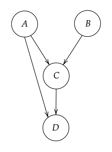
A small DAG with four nodes

Nodes $A$ and $B$ are root nodes because they do not have any directed edges pointing into them. Nodes $C$ and $D$ on the other hand are child nodes. The parents of node $C$ are both $A$ and $B$ because both of these nodes have directed edge towards $C$ . Note that node $B$ is not a parent of node $D$ because there is no edge from $B$ to $D$ .

As the name implies, DAGs do not have cycles. Therefore every DAG has at least one root node. Generating data for these nodes is the first step to simulate data for the whole DAG. Since root nodes have no parents, we can simply generate random data from them using an appropriate distribution. Once we have data for all root nodes, we can generate their directly connected child nodes next as a function of the root nodes (and perhaps additional random error). These direct child nodes are then used as input for the next child nodes in line and so on. This continues until every node has been generated. Since every DAG can be topologically sorted (Chickering 1995), this will always work. All we need is to specify the DAG and the functional relationship between each node and its parents.

Defining the DAG

Because the sim_from_dag() function uses the method described above, it requires information about the causal structure and the exact form of the relationship between child nodes and their parents. All of this information has to be included in the dag argument, which should be a DAG object created using the empty_dag() function and grown using node() calls as described below. This can be done completely manually (which is the usual strategy when conducting simulation studies) or (partially) using existing data (which may be useful when the interest is in getting a toy data set resembling real data as closely as possible).

Regardless of which strategy you want to use, first you have to initialize an empty DAG object like this:

library(data.table)
library(ggplot2)
#> Error in get(paste0(generic, ".", class), envir = get_method_env()) : 
#>   object 'type_sum.accel' not found
library(simDAG)

dag <- empty_dag()

Afterwards you can add an unlimited amount of root nodes and child nodes to it. Multiple different types are implemented.

Root node types

The values for the root_nodes are simply sampled from some defined distributions. Therefore, any function that generates random draws from some distribution may be used here. Popular alternatives for continuous data are the normal-, beta-, gamma-distributions which are implemented in base R inside the rnorm(), rbeta() and rgamma() functions. For binary or categorical data we could use the custom functions rbernoulli() or rcategorical() instead.

Child node types

The simDAG package implements the following types of child_nodes directly:

node_gaussian: A node based on linear regression (continuous data).
node_binomial: A node based on logistic regression (binary data).
node_multinomial: A node based on multinomial logistic regression (categorical data).
node_poisson: A node based on poisson regression (count data).
node_negative_binomial: A node based on negative binomial regression (count data).
node_cox: A node based on cox regression (time-to-event data).
node_conditional_prob: A node based on conditional probabilities (binary / categorical data).
node_conditional_distr: A node based on conditional distributions (any data type).
node_identity: A node that is just some R expression of other nodes (any data type).

All of these nodes have their own documentation page containing a detailed description on how data is generated from them. Although this collection of nodes covers a lot of data types, it is still a somewhat limited collection. If, for example, we wanted to add a child node that is normally distributed but also truncated at specific values, we could not do this using just the offered node functions. For this reason, the sim_from_dag() function also allows the user to use custom functions as nodes, which makes it possible to model any kind of data and any kind of relationship.

Defining nodes manually

Suppose that node $A$ in the figure above stands for age, $B$ stands for sex, $C$ stands for the Body-Mass-Index (BMI) and $D$ stands for death. We have to start by defining what the root nodes should look like. We use the following code to define age and sex:

dag <- dag + 
  node("age", type="rnorm", mean=50, sd=4) +
  node("sex", type="rbernoulli", p=0.5)

All nodes are defined by calling the node() function and adding the output to the dag object using a simple +. This syntax is heavily inspired by the simCausal R-package (Sofrygin et al. 2017). Here, we assume that age is a continuous normally distributed variable with a mean of 50 and a standard deviation of 4 (If this was a real simulation study we would probably use a truncated normal distribution to ensure that age is not negative). This can be done by setting the dist parameter to "rnorm", which is the standard R function for generating random values from a normal distribution. All arguments listed in the params parameter will be passed to this function. Similarly, we define sex to be a Bernoulli distributed variable (taking only the values 0/1). We assume that there is an even gender distribution by setting p = 0.5.

Next, we have to define what the relationship between the child nodes and their parents should look like. We may use the following code:

dag <- dag +
  node("bmi", type="gaussian", parents=c("sex", "age"), betas=c(1.1, 0.4),
       intercept=12, error=2) +
  node("death", type="binomial", parents=c("age", "bmi"), betas=c(0.1, 0.3),
       intercept=-15)

Since the bmi node is dependent on both sex and age, we have to list both of these nodes as the parents of bmi. We then specify that the bmi should be a continuous variable modeled using a linear regression by setting type="gaussian". The concrete regression equation is defined through the use of the intercept, betas and error arguments. Our specification for the bmi node corresponds to the following equation:

$bmi = 12 + sex \cdot 1.1 + age \cdot 0.4 + N(0, 2),$

where $N(0, 2)$ indicates that the error term is modelled as a normally distributed variable with mean 0 and a standard deviation of 2.

Since death has only two states (alive vs. dead), we use a logistic regression model here instead. We can do this easily by setting type="binomial". The rest of the syntax essentially stays the same. The regression equation for death as described by the code above is then:

$logit(death) = -15 + age \cdot 0.1 + bmi \cdot 0.3.$

To check whether we got the causal relationships right, we can call the plot() function on the DAG object. The output should look very similar to the hand-drawn DAG above.

plot(dag)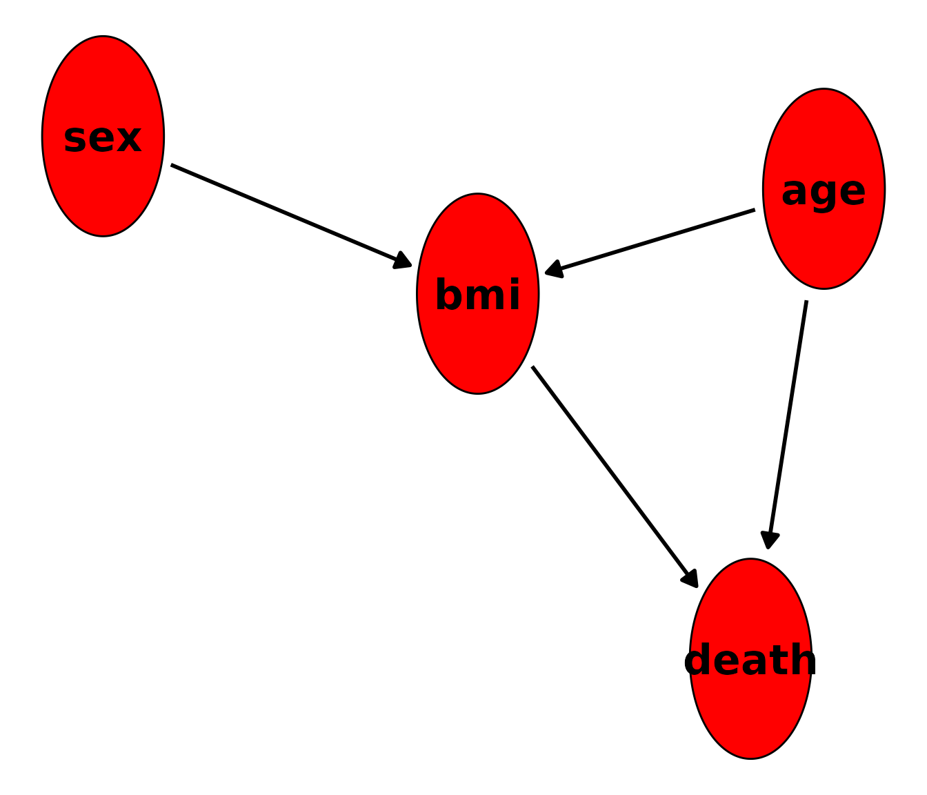
#> Loading required namespace: ggforce

We can also directly print the underlying structural equations using the summary() function:

summary(dag)
#> A DAG object using the following structural equations:
#> 
#>   age ~ N(50, 4)
#>   sex ~ Bernoulli(0.5)
#>   bmi ~ N(12 + 1.1*sex + 0.4*age, 2)
#> death ~ Bernoulli(logit(-15 + 0.1*age + 0.3*bmi))

This is all correct. We can now use this DAG object to generate random data using the sim_from_dag() function:

set.seed(42)
sim_dat <- sim_from_dag(dag=dag, n_sim=10000)

Setting a seed for the random number generator is necessary to obtain replicable results. The data generated using this code looks like this:

head(sim_dat, 5)
#>         age    sex      bmi  death
#>       <num> <lgcl>    <num> <lgcl>
#> 1: 55.48383   TRUE 33.25311  FALSE
#> 2: 47.74121  FALSE 29.58815  FALSE
#> 3: 51.45251  FALSE 30.12967  FALSE
#> 4: 52.53145   TRUE 32.07877  FALSE
#> 5: 51.61707  FALSE 36.09082   TRUE

Binary variables such as sex and death are by default treated as logical variables, because this is the most memory efficient way to store them. We can now check the distributions and relationships in this dataset to confirm that it indeed corresponds to our specified causal DAG. Starting with the root nodes:

hist(sim_dat$age)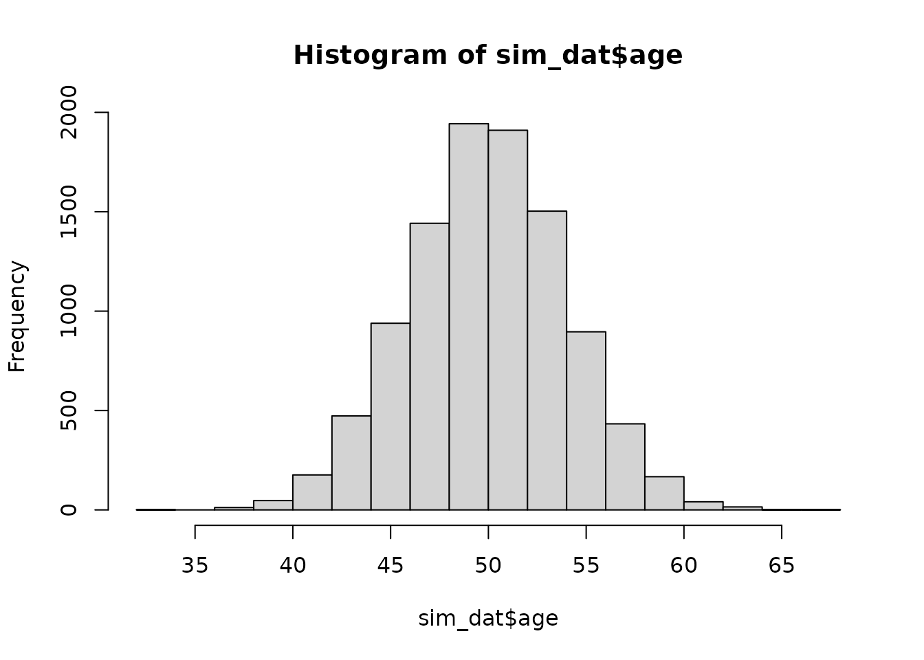

table(sim_dat$sex)
#> 
#> FALSE  TRUE 
#>  5051  4949

This seems to be correct. Note that this is a finite dataset, which means that the results will never exactly match the theoretical distributions. But it’s definitely close enough here. To check if the child nodes were modeled correctly, we simply fit the corresponding models using the glm() function:

mod_bmi <- glm(bmi ~ age + sex, data=sim_dat, family="gaussian")
summary(mod_bmi)
#> 
#> Call:
#> glm(formula = bmi ~ age + sex, family = "gaussian", data = sim_dat)
#> 
#> Coefficients:
#>              Estimate Std. Error t value Pr(>|t|)    
#> (Intercept) 12.184254   0.253188   48.12   <2e-16 ***
#> age          0.396020   0.005039   78.58   <2e-16 ***
#> sexTRUE      1.177159   0.040563   29.02   <2e-16 ***
#> ---
#> Signif. codes:  0 '***' 0.001 '**' 0.01 '*' 0.05 '.' 0.1 ' ' 1
#> 
#> (Dispersion parameter for gaussian family taken to be 4.112615)
#> 
#>     Null deviance: 70134  on 9999  degrees of freedom
#> Residual deviance: 41114  on 9997  degrees of freedom
#> AIC: 42524
#> 
#> Number of Fisher Scoring iterations: 2

mod_death <- glm(death ~ age + bmi, data=sim_dat, family="binomial")
summary(mod_death)
#> 
#> Call:
#> glm(formula = death ~ age + bmi, family = "binomial", data = sim_dat)
#> 
#> Coefficients:
#>               Estimate Std. Error z value Pr(>|z|)    
#> (Intercept) -14.319144   0.371511  -38.54   <2e-16 ***
#> age           0.093229   0.007057   13.21   <2e-16 ***
#> bmi           0.289714   0.011331   25.57   <2e-16 ***
#> ---
#> Signif. codes:  0 '***' 0.001 '**' 0.01 '*' 0.05 '.' 0.1 ' ' 1
#> 
#> (Dispersion parameter for binomial family taken to be 1)
#> 
#>     Null deviance: 13773  on 9999  degrees of freedom
#> Residual deviance: 11805  on 9997  degrees of freedom
#> AIC: 11811
#> 
#> Number of Fisher Scoring iterations: 3

Evidently, the coefficients do match the causal coefficients we specified earlier.

Defining nodes using existing data

If the data should resemble a specific real data set, it makes sense to base the values for the causal coefficients on that specific data set. This can be done by fitting a single model for each child node, extracting the estimated coefficients from the fitted models and putting those into an appropriate DAG object. If the assumed DAG is big, this can be a time-extensive task. The dag_from_data() function automates this process. This function takes a node list containing only minimal information about the causal structure and node type and outputs a fully specified DAG object.

For example, lets assume that the data we just generated (sim_dat) was our data set of interest. Let us also assume that we know the true underlying causal diagram and have a rough idea about the nature of the relationship between the nodes (e.g. we know or can reasonably guess the node type). Now all we have to do is create a partially specified DAG in accordance to these assumptions first:

dag <- empty_dag() +
  node("age", type="rnorm") +
  node("sex", type="rbernoulli") +
  node("bmi", type="gaussian", parents=c("sex", "age")) +
  node("death", type="binomial", parents=c("age", "bmi"))

This looks a lot like the code used above, except that we are not explicitly defining the actual beta coefficients. We only define the causal structure and the node types. Now we can call the dag_from_data() function:

est_dag <- dag_from_data(dag=dag, data=sim_dat)

It returns an object that includes a fully specified DAG, which can be used directly in the sim_from_dag() function:

sim_dat2 <- sim_from_dag(dag=est_dag$dag, n_sim=10000)

The dag_from_data() function essentially just fits the corresponding models one by one for each node and extracts the relevant data from the models to fill in the gaps in the empty nodes. If we set return_models to TRUE in the dag_from_data() function call above, we can actually see that it used the exact same models we fit earlier to check if the simulation was valid.

Time-varying covariates

Most real data sets include time-varying covariates, e.g. variables that are measured at multiple points in time that are subject to changes. It is possible to generate this type of data using the sim_from_dag() function as well. All we need to do is to define an appropriate DAG that directly specifies how the variables change over time. For example, we can extend the simple DAG from above to include a dimension of time:

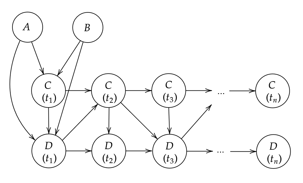
A small DAG with four nodes

Here, nodes $A$ and $B$ are time-constant variables that only have a causal effect on the initial state of $C$ and $D$ , while nodes $C$ and $D$ change over time interdependently. If we want to simulate data from a DAG that looks like this using the sim_from_dag() function, we have to add a node to the for every point in time that we want to consider.

We will quickly go through a somewhat simpler example, considering only 2 points in time. We define our nodes in the following way:

dag <- empty_dag() +
  node("age", type="rnorm", mean=50, sd=4) +
  node("sex", type="rbernoulli", p=0.5) +
  node("bmi_t1", type="gaussian", betas=c(1.1, 0.4), parents=c("sex", "age"),
       intercept=12, error=2) +
  node("death_t1", type="binomial", parents=c("age", "sex", "bmi_t1"),
       betas=c(0.1, 0.3, 0.1), intercept=-15) +
  node("bmi_t2", type="gaussian", parents="bmi_t1", betas=c(1.1), intercept=0,
       error=2) +
  node("death_t2", type="binomial", betas=c(0.1, 0.3),
       parents=c("age", "bmi_t2"), intercept=-15)

sim_dat <- sim_from_dag(dag=dag, n_sim=10000)

In this example, the bmi at $t = 1$ is a function of both sex and age, but the bmi at $t = 2$ is only a function of the previous bmi. The death node is determined by the initial age and by the time-varying bmi. This surely is not the most realistic example. It is only meant to show how the sim_from_dag() function may be used to incorporate time-dependent covariates. If many points in time should be considered or there are very complex time-dependent structures that may not be easily described using a DAG like the one above, the sim_discrete_time() function also included in this package may be used instead.

References

Judea Pearl (2009). Causality: Models, Reasoning and Inference. 2nd ed. Cambridge: Cambridge University Press

Peter Spirtes, Clark Glymour, and Richard Scheines (2000) Causation, Prediction, and Search. 2nd ed. The MIT Press, Cambridge

Chickering, D.M. (1995). A transformational characterization of equivalent Bayesian network structures. Proceedings of the 11th Conference on Uncertainty in Artificial Intelligence, Montreal, Canada, 87-98.

Oleg Sofrygin, Mark J. van der Laan, and Romain Neugebauer (2017). simcausal R Package: Conducting Transparent and Reproducible Simulation Studies of Causal Effect Estimation with Complex Longitudinal Data. In: Journal of Statistical Software. 81.2, pp. 1-47

Robin Denz

References

Denz, Robin and Nina Timmesfeld (2025). Simulating Complex Crossectional and Longitudinal Data using the simDAG R Package. arXiv preprint, doi: 10.48550/arXiv.2506.01498.