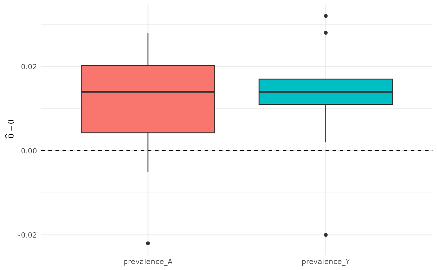
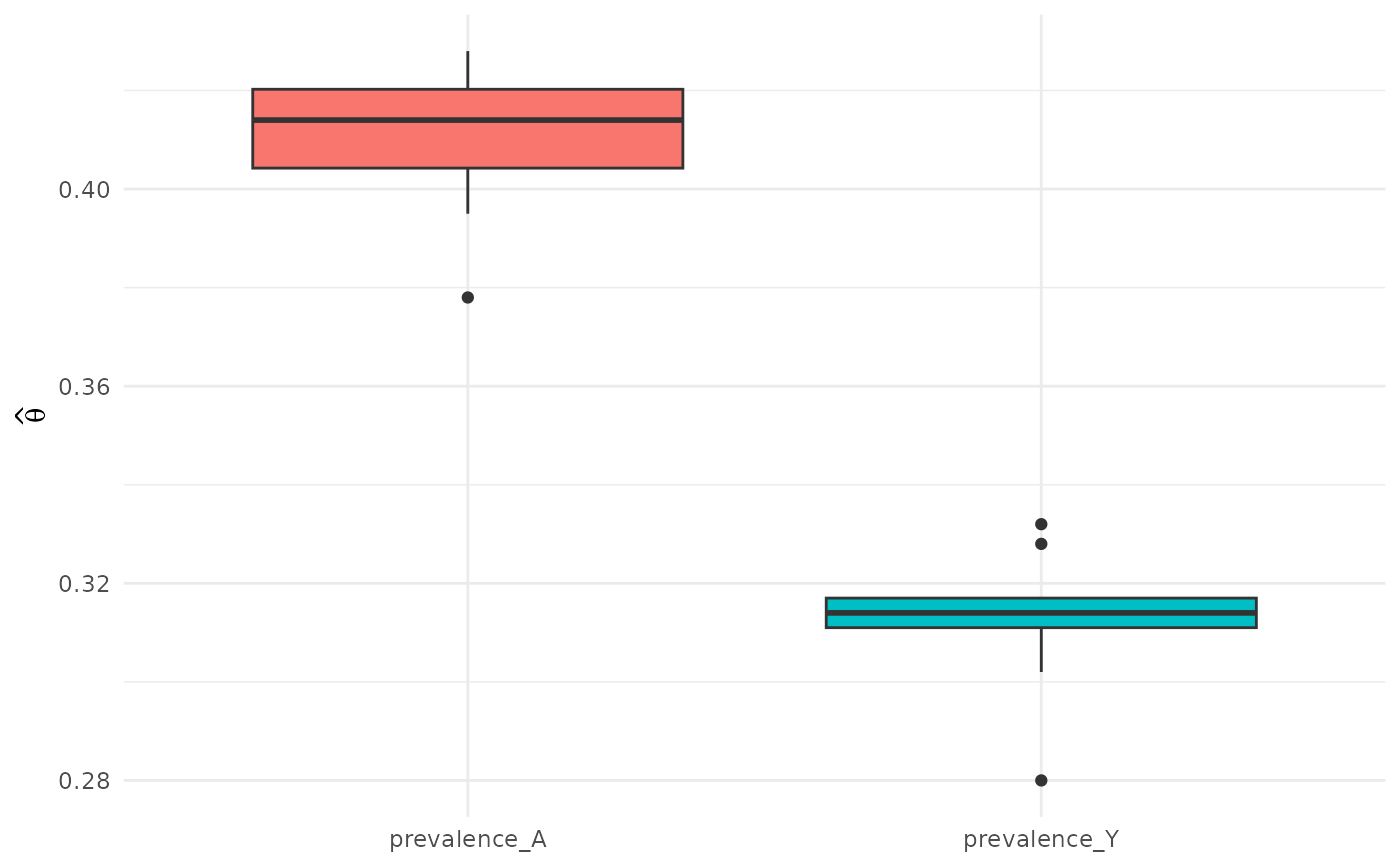
Plot a calibrated_DAG object — plot.calibrated

This function may be used to visually inspect how well a calibrate_dag function call was able to approximate the desired targets. If fitted with n_reps_eval > 1, it plots the distribution of the targets estimated on the n_reps_eval evaluation datasets using the determined parameters. Alternatively plots the bias directly.

Usage

# S3 method for class 'calibrated_DAG'
plot(x, type="errors", xlab=NULL,
     ylab="auto", line_at_0=TRUE, ...)

Arguments

x: A calibrated_DAG object created using the calibrate_dag function.
type: A single character string, specifying what should be plotted. Should be either "targets" (to plot the raw target estimates), "scaled_targets" (to plot the target estimates after applying the user-specified scaling factors, if applicable), "errors" (to plot the difference between the estimated targets and the desired targets, the default) or "scaled_errors" (same as errors, but after applying the user-specified scaling factors, if applicable).
xlab: A single character string specifying the name of the x-axis or NULL (default) to not use a name.
ylab: A single character string specifying the name of the y-axis or NULL to not use a name. If set to "auto" (default), the label will be determined automatically based on the supplied type.
line_at_0: Either TRUE or FALSE, specifying whether to plot a dashed line at 0 whenever type = "errors" or type = "scaled_errors" is used, ignored otherwise.
...: Further arguments passed to the geom_boxplot function, allowing users to customize their appearance further.

Details

The function internally relies on the ggplot2 package, so any further ggplot2 syntax may be used to customize the plot. Its main use is to visually assess whether the observed discrepancy between the estimated and desired targets is due to sampling error or a genuine difference.

Author

Robin Denz

Value

Returns a standard ggplot2 object.

Examples

# Jointly calibrate treatment and outcome prevalence.
# The DAG contains two free parameters and two targets.
# Parameter ranges are optional.

ldag <- lazy_dag(
  empty_dag() +
    node("X", type="rnorm") +
    node("A", type="binomial",
         formula= ~ param(intercept_A) + X * 0.5) +
    node("Y", type="binomial",
         formula= ~ param(intercept_Y) + A * 0.7 + X * 0.4)
)

targets <- list(
  prevalence_A = list(
    target = 0.4,
    eval_fun = function(data) mean(data$A)
  ),
  prevalence_Y = list(
    target = 0.3,
    eval_fun = function(data) mean(data$Y)
  )
)

params <- list(
  intercept_A = list(start = 0),
  intercept_Y = list(start = 0)
)

fit <- calibrate_dag(
  lazy_dag = ldag,
  targets = targets,
  params = params,
  n_sim_run = 2000,
  n_sim_eval = 1000,
  n_reps_eval = 10,
  seed = 123,
  optim_control = list(
    maxit = 200,
    trace = 0,
    ndeps = c(0.05, 0.05),
    factr = 100
  )
)
summary(fit)
#> ────────────────────────────────────────────────────────────
#> Calibrated DAG
#> ────────────────────────────────────────────────────────────
#> Parameters (2)
#>    parameter estimate start lower upper parscale
#>  intercept_A  -0.3828     0  -Inf   Inf        1
#>  intercept_Y  -1.1368     0  -Inf   Inf        1
#> 
#> Targets (2)
#>        target desired achieved  error scaled_error
#>  prevalence_A     0.4   0.4104 0.0104       0.0104
#>  prevalence_Y     0.3   0.3126 0.0126       0.0126
#> 
#> Optimization
#>   Optimizer:    optim()
#>   Method:       L-BFGS-B
#>   Convergence:  unsuccessful (code 52)
#>   Objective:    5e-07
#>   Evaluations:  function 47, gradient 47
#>   Message:      ERROR: ABNORMAL_TERMINATION_IN_LNSRCH
#>   Simulations:  2,000 optimization; 1,000 final evaluation
#> ────────────────────────────────────────────────────────────

# plot the targets directly
plot(fit, type="targets")


# plot the errors instead
plot(fit, type="errors")